| .. | ||
| datasets | ||
| dllogger | ||
| images | ||
| model | ||
| notebooks | ||
| runtime | ||
| scripts | ||
| utils | ||
| .gitignore | ||
| Dockerfile | ||
| download_and_preprocess_dagm2007.sh | ||
| download_and_preprocess_dagm2007_public.sh | ||
| export_saved_model.py | ||
| LICENSE | ||
| main.py | ||
| NOTICE | ||
| preprocess_dagm2007.py | ||
| README.md | ||
U-Net Industrial Defect Segmentation for TensorFlow
This repository provides a script and recipe to train U-Net Industrial to achieve state of the art accuracy on the dataset DAGM2007, and is tested and maintained by NVIDIA.
Table of Contents
Model overview
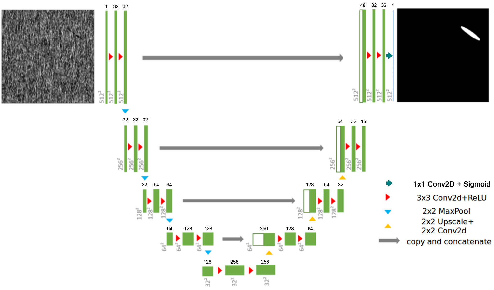
This U-Net model is adapted from the original version of the U-Net model which is a convolutional auto-encoder for 2D image segmentation. U-Net was first introduced by Olaf Ronneberger, Philip Fischer, and Thomas Brox in the paper: U-Net: Convolutional Networks for Biomedical Image Segmentation.
This work proposes a modified version of U-Net, called TinyUNet which performs efficiently and with very high accuracy
on the industrial anomaly dataset DAGM2007.
TinyUNet, like the original U-Net is composed of two parts:
- an encoding sub-network (left-side)
- a decoding sub-network (right-side).
It repeatedly applies 3 downsampling blocks composed of two 2D convolutions followed by a 2D max pooling layer in the encoding sub-network. In the decoding sub-network, 3 upsampling blocks are composed of a upsample2D layer followed by a 2D convolution, a concatenation operation with the residual connection and two 2D convolutions.
TinyUNet has been introduced to reduce the model capacity which was leading to a high degree of over-fitting on a
small dataset like DAGM2007. The complete architecture is presented in the figure below:
This model trains with mixed precision tensor cores on Volta, therefore researchers can get results much faster than training without tensor cores. This model is tested against each NGC monthly container release to ensure consistent accuracy and performance over time.
The following features were implemented in this model:
- Data-parallel multi-GPU training with Horovod.
- Mixed precision support with TensorFlow Automatic Mixed Precision (TF-AMP), which enables mixed precision training without any changes to the code-base by performing automatic graph rewrites and loss scaling controlled by an environmental variable.
- Tensor Core operations to maximize throughput using NVIDIA Volta GPUs.
- Loss auto-scaling for Tensor Cores (mixed precision) training
The following performance optimizations were implemented in this model:
- XLA support (experimental)
Default Configuration
This model trains in 2500 epochs, under the following setup:
-
Global Batch Size: 16
-
Optimizer RMSProp:
- decay: 0.9
- momentum: 0.8
- centered: True
-
Learning Rate Schedule: Exponential Step Decay
- decay: 0.8
- steps: 500
- initial learning rate: 1e-4
-
Weight Initialization: He Uniform Distribution (introduced by Kaiming He et al. in 2015 to address issues related ReLU activations in deep neural networks)
-
Loss Function: Adaptive
- When DICE Loss < 0.3, Loss = Binary Cross Entropy
- Else, Loss = DICE Loss
-
Data Augmentation
- Random Horizontal Flip (50% chance)
- Random Rotation 90°
-
Activation Functions:
- ReLU is used for all layers
- Sigmoid is used at the output to ensure that the ouputs are between [0, 1]
-
Weight decay: 1e-5
Enabling mixed precision
Mixed precision training offers significant computational speedup by performing operations in half-precision format, while storing minimal information in single-precision to retain as much information as possible in critical parts of the network. Since the introduction of tensor cores in the Volta and Turing architectures, significant training speedups are experienced by switching to mixed precision -- up to 3x overall speedup on the most arithmetically intense model architectures. Using mixed precision training previously required two steps:
- Porting the model to use the FP16 data type where appropriate.
- Manually adding loss scaling to preserve small gradient values.
This can now be achieved using Automatic Mixed Precision (AMP) for TensorFlow to enable the full mixed precision methodology in your existing TensorFlow model code. AMP enables mixed precision training on Volta and Turing GPUs automatically. The TensorFlow framework code makes all necessary model changes internally.
In TF-AMP, the computational graph is optimized to use as few casts as necessary and maximize the use of FP16, and the loss scaling is automatically applied inside of supported optimizers. AMP can be configured to work with the existing tf.contrib loss scaling manager by disabling the AMP scaling with a single environment variable to perform only the automatic mixed-precision optimization. It accomplishes this by automatically rewriting all computation graphs with the necessary operations to enable mixed precision training and automatic loss scaling.
For information about:
- How to train using mixed precision, see the Mixed Precision Training paper and Training With Mixed Precision documentation.
- How to access and enable AMP for TensorFlow, see Using TF-AMP from the TensorFlow User Guide.
- Techniques used for mixed precision training, see the Mixed-Precision Training of Deep Neural Networks blog.
Setup
The following section list the requirements in order to start training the U-Net model
(only the TinyUnet model is proposed here).
Requirements
This repository contains Dockerfile which extends the TensorFlow NGC container and encapsulates some dependencies.
Aside from these dependencies, ensure you have the following components:
-
(optional) NVIDIA Volta GPU (see section below) - for best training performance using mixed precision
For more information about how to get started with NGC containers, see the following sections from the NVIDIA GPU Cloud Documentation and the Deep Learning Documentation:
- Getting Started Using NVIDIA GPU Cloud,
- Accessing And Pulling From The NGC container registry
- Running TensorFlow.
Quick Start Guide
To train your model using mixed precision with tensor cores or using FP32, perform the following steps using the
default configuration of the U-Net model (only TinyUNet has been made available here) on the DAGM2007 dataset.
Clone the repository
git clone https://github.com/NVIDIA/DeepLearningExamples
cd DeepLearningExamples/TensorFlow/Segmentation/UNetIndustrial
Download and preprocess the dataset: DAGM2007
In order to download the dataset. You can execute the following:
./download_and_preprocess_dagm2007.sh /path/to/dataset/directory/
Important Information: Some files of the dataset require an account to be downloaded, the script will invite you to download them manually and put them in the correct directory.
Build and start the docker container based on the TensorFlow NGC container.
# Build the docker container
docker build . --rm -t unet_industrial:latest

# start the container with nvidia-docker
nvidia-docker run -it --rm \
    --shm-size=2g --ulimit memlock=-1 --ulimit stack=67108864 \
    -v /path/to/dataset:/data/dagm2007/ \
    -v /path/to/results:/results \
    unet_industrial:latest
Run training
To run training for a default configuration (as described in Default configuration, for example 1/4/8 GPUs,
FP32/TF-AMP), launch one of the scripts in the ./scripts directory called
./scripts/UNet_{FP32, AMP}_{1, 4, 8}GPU.sh
Each of the scripts requires three parameters:
- path to the result directory of the model as the first argument
- path to the dataset as a second argument
- class ID from DAGM used (between 1-10)
For example:
cd scripts/
./UNet_FP32_1GPU.sh <path to result repository> <path to dataset> <DAGM2007 classID (1-10)>
Run evaluation
Model evaluation on a checkpoint can be launched by running one of the scripts in the ./scripts directory
called ./scripts/UNet_{FP32, AMP}_EVAL.sh.
Each of the scripts requires three parameters:
- path to the result directory of the model as the first argument
- path to the dataset as a second argument
- class ID from DAGM used (between 1-10)
For example:
cd scripts/
./UNet_FP32_EVAL.sh <path to result repository> <path to dataset> <DAGM2007 classID (1-10)>
If you wish to evaluate external checkpoint, make sure to put the TF ckpt files inside a folder named "checkpoints"
and provide its parent path as <path to result repository> in the example above.
Be aware that the script will not fail if it does not find the checkpoint.
It will randomly initialize the weights and run performance tests.
Advanced
The following sections provide greater details of the dataset, running training and inference, and the training results.
Command line options
To see the full list of available options and their descriptions, use the -h or --help command line option, for example:
python main.py --help
The following mandatory flags must be used to tune different aspects of the training:
general
--exec_mode=train_and_evaluate Which execution mode to run the model into.
--iter_unit=batch Will the model be run for X batches or X epochs ?
--num_iter=2500 Number of iterations to run.
--batch_size=16 Size of each minibatch per GPU.
--results_dir=/path/to/results Directory in which to write training logs, summaries and checkpoints.
--data_dir=/path/to/dataset Directory which contains the DAGM2007 dataset.
--dataset_name=DAGM2007 Name of the dataset used in this run (only DAGM2007 is supported atm).
--dataset_classID=1 ClassID to consider to train or evaluate the network (used for DAGM).
model
--use_tf_amp Enable Automatic Mixed Precision to speedup FP32 computation using tensor cores.
--use_xla Enable TensorFlow XLA to maximise performance.
--use_auto_loss_scaling Use AutoLossScaling in TF-AMP
Getting the data
The U-Net model was trained with the Weakly Supervised Learning for Industrial Optical Inspection (DAGM 2007) dataset.
The competition is inspired by problems from industrial image processing. In order to satisfy their customers' needs, companies have to guarantee the quality of their products, which can often be achieved only by inspection of the finished product. Automatic visual defect detection has the potential to reduce the cost of quality assurance significantly.
The competitors have to design a stand-alone algorithm which is able to detect miscellaneous defects on various background textures.
The particular challenge of this contest is that the algorithm must learn, without human intervention, to discern defects automatically from a weakly labeled (i.e., labels are not exact to the pixel level) training set, the exact characteristics of which are unknown at development time. During the competition, the programs have to be trained on new data without any human guidance.
Source: https://resources.mpi-inf.mpg.de/conference/dagm/2007/prizes.html
Data description
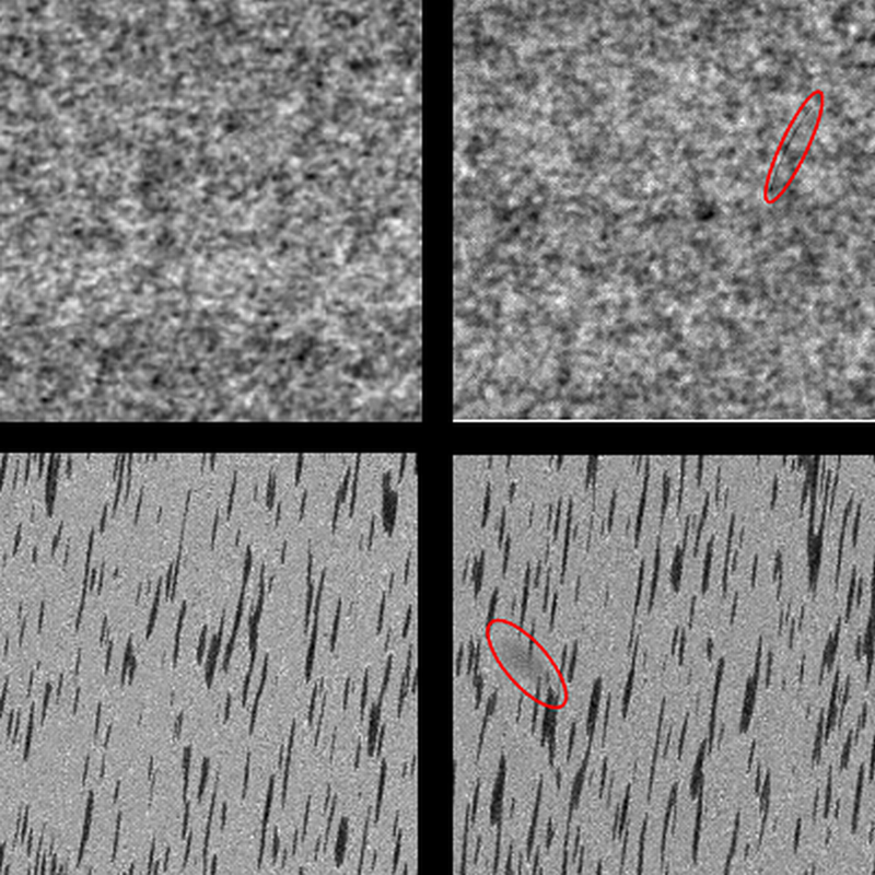
The provided data is artificially generated, but similar to real world problems. It consists of multiple data sets, each consisting of 1000 images showing the background texture without defects, and of 150 images with one labeled defect each on the background texture. The images in a single data set are very similar, but each data set is generated by a different texture model and defect model.
Not all deviations from the texture are necessarily defects. The algorithm will need to use the weak labels provided during the training phase to learn the properties that characterize a defect.
Below are two sample images from two data sets. In both examples, the left images are without defects; the right ones contain a scratch-shaped defect which appears as a thin dark line, and a diffuse darker area, respectively. The defects are weakly labeled by a surrounding ellipse, shown in red.
The DAGM2007 challenge comes in propose two different challenges:
- A development set: public and available for download from here. The number of classes and sub-challenges for the development set is 6.
- A competition set: which requires an account to be downloaded from here. The number of classes and sub-challenges for the competition set is 10.
Challenge description
The challenge consists in designing a single model with a set of predefined hyper-parameters which will not change across the 10 different classes or sub-challenges of the competition set.
The performance shall be measured on the competition set which is normalized and more complex that the public dataset while offering the most unbiased evaluation method.
Training Process
Laplace Smoothing
We use this technique in the DICE loss to improve the training efficiency. This technique consists in replacing the epsilon parameter (used to avoid dividing by zero and very small: +/- 1e-7) by 1. You can find more information on: https://en.wikipedia.org/wiki/Additive_smoothing
Adaptive Loss
The DICE Loss is not able to provide a meaningful gradient at initialisation. This leads to a model instability which often push the model to diverge. Nonetheless, once the model starts to converge, DICE loss is able to very efficiently fully train the model. Therefore, we implemented an adaptive loss which is composed of two sub-losses:
- Binary Cross-Entropy (BCE)
- DICE Loss
The model is trained with the BCE loss until the DICE Loss reach a experimentally defined threshold (0.3). Thereafter, DICE loss is used to finish training.
Weak Labelling
This dataset is referred as weakly labelled. That means that the segmentation labels are not given at the pixel level but rather in an approximate fashion.
Performance
Benchmarking
The following sections shows how to run benchmarks measuring the model performance in training and inference modes.
Training performance benchmark
To benchmark the inference performance, you can run one of the scripts in the ./scripts/benchmarking/ directory
called ./scripts/benchmarking/DGX1v_trainbench_{FP32, AMP}_{1, 4, 8}GPU.sh.
Each of the scripts requires three parameters:
- path to the result directory of the model as the first argument
- path to the dataset as a second argument
- class ID from DAGM used (between 1-10)
For example:
cd scripts/benchmarking/
./DGX1v_trainbench_FP32_1GPU.sh <path to result repository> <path to dataset> <DAGM2007 classID (1-10)>
Inference performance benchmark
To benchmark the training performance, you can run one of the scripts in the ./scripts/benchmarking/ directory
called ./scripts/benchmarking/DGX1v_trainbench_{FP32, AMP}_{1, 4, 8}GPU.sh.
Each of the scripts requires three parameters:
- path to the result directory of the model as the first argument
- path to the dataset as a second argument
- class ID from DAGM used (between 1-10)
For example:
cd scripts/benchmarking/
./DGX1v_evalbench_FP16_1GPU.sh <path to result repository> <path to dataset> <dagm classID (1-10)>
Results
The following sections provide details on the achieved results in training accuracy, performance and inference performance.
Training accuracy results
Our results were obtained by running the ./scripts/UNet_{FP32, AMP}_{1, 4, 8}GPU.sh training
script in the Tensorflow:19.03-py3 NGC container on NVIDIA DGX-1 with 8x V100 16G GPUs.
Threshold = 0.75
| # DAGM Class ID | Precision | IoU (Intersection over Union) | TPR (True Positive Rate) | TNR (True Negative Rate) |
|---|---|---|---|---|
| 1 | FP32 | 0.968 | 100.00 | 97.88 |
| 1 | Automatic Mixed Precision (AMP) | 0.966 | 100.00 | 97.55 |
| 2 | FP32 | 0.976 | 100.00 | 99.62 |
| 2 | Automatic Mixed Precision (AMP) | 0.976 | 100.00 | 99.66 |
| 3 | FP32 | 0.979 | 100.00 | 99.64 |
| 3 | Automatic Mixed Precision (AMP) | 0.979 | 100.00 | 99.63 |
| 4 | FP32 | 0.965 | 100.00 | 97.43 |
| 4 | Automatic Mixed Precision (AMP) | 0.960 | 100.00 | 96.85 |
| 5 | FP32 | 0.992 | 100.00 | 99.88 |
| 5 | Automatic Mixed Precision (AMP) | 0.991 | 100.00 | 99.78 |
| 6 | FP32 | 0.982 | 100.00 | 98.78 |
| 6 | Automatic Mixed Precision (AMP) | 0.979 | 100.00 | 98.39 |
| 7 | FP32 | 0.980 | 100.00 | 99.58 |
| 7 | Automatic Mixed Precision (AMP) | 0.980 | 100.00 | 99.56 |
| 8 | FP32 | 0.970 | 100.00 | 99.85 |
| 8 | Automatic Mixed Precision (AMP) | 0.971 | 100.00 | 100.00 |
| 9 | FP32 | 0.988 | 99.82 | 99.81 |
| 9 | Automatic Mixed Precision (AMP) | 0.988 | 99.87 | 99.81 |
| 10 | FP32 | 0.979 | 100.00 | 99.43 |
| 10 | Automatic Mixed Precision (AMP) | 0.982 | 100.00 | 99.70 |
Threshold = 0.85
| # DAGM Class ID | Precision | IoU (Intersection over Union) | TPR (True Positive Rate) | TNR (True Negative Rate) |
|---|---|---|---|---|
| 1 | FP32 | 0.968 | 100.00 | 97.88 |
| 1 | Automatic Mixed Precision (AMP) | 0.966 | 100.00 | 97.56 |
| 2 | FP32 | 0.976 | 100.00 | 99.62 |
| 2 | Automatic Mixed Precision (AMP) | 0.976 | 100.00 | 99.66 |
| 3 | FP32 | 0.979 | 100.00 | 99.64 |
| 3 | Automatic Mixed Precision (AMP) | 0.977 | 100.00 | 99.33 |
| 4 | FP32 | 0.966 | 100.00 | 97.44 |
| 4 | Automatic Mixed Precision (AMP) | 0.960 | 100.00 | 96.85 |
| 5 | FP32 | 0.992 | 100.00 | 99.88 |
| 5 | Automatic Mixed Precision (AMP) | 0.991 | 100.00 | 99.78 |
| 6 | FP32 | 0.982 | 100.00 | 98.80 |
| 6 | Automatic Mixed Precision (AMP) | 0.979 | 100.00 | 98.41 |
| 7 | FP32 | 0.980 | 100.00 | 99.60 |
| 7 | Automatic Mixed Precision (AMP) | 0.980 | 100.00 | 99.58 |
| 8 | FP32 | 0.970 | 100.00 | 99.85 |
| 8 | Automatic Mixed Precision (AMP) | 0.971 | 100.00 | 100.00 |
| 9 | FP32 | 0.988 | 99.82 | 99.81 |
| 9 | Automatic Mixed Precision (AMP) | 0.988 | 99.87 | 99.81 |
| 10 | FP32 | 0.980 | 100.00 | 99.45 |
| 10 | Automatic Mixed Precision (AMP) | 0.982 | 100.00 | 99.71 |
Threshold = 0.95
| # DAGM Class ID | Precision | IoU (Intersection over Union) | TPR (True Positive Rate) | TNR (True Negative Rate) |
|---|---|---|---|---|
| 1 | FP32 | 0.969 | 100.00 | 97.93 |
| 1 | Automatic Mixed Precision (AMP) | 0.966 | 100.00 | 97.58 |
| 2 | FP32 | 0.976 | 100.00 | 99.64 |
| 2 | Automatic Mixed Precision (AMP) | 0.976 | 100.00 | 99.66 |
| 3 | FP32 | 0.979 | 100.00 | 99.64 |
| 3 | Automatic Mixed Precision (AMP) | 0.980 | 100.00 | 99.64 |
| 4 | FP32 | 0.966 | 100.00 | 97.52 |
| 4 | Automatic Mixed Precision (AMP) | 0.961 | 100.00 | 96.88 |
| 5 | FP32 | 0.992 | 100.00 | 99.88 |
| 5 | Automatic Mixed Precision (AMP) | 0.991 | 100.00 | 99.78 |
| 6 | FP32 | 0.982 | 100.00 | 98.83 |
| 6 | Automatic Mixed Precision (AMP) | 0.980 | 100.00 | 98.58 |
| 7 | FP32 | 0.981 | 100.00 | 99.65 |
| 7 | Automatic Mixed Precision (AMP) | 0.980 | 100.00 | 99.59 |
| 8 | FP32 | 0.970 | 100.00 | 99.88 |
| 8 | Automatic Mixed Precision (AMP) | 0.971 | 100.00 | 100.00 |
| 9 | FP32 | 0.988 | 99.82 | 99.83 |
| 9 | Automatic Mixed Precision (AMP) | 0.988 | 99.87 | 99.82 |
| 10 | FP32 | 0.980 | 100.00 | 99.54 |
| 10 | Automatic Mixed Precision (AMP) | 0.982 | 100.00 | 99.72 |
Threshold = 0.99
| # DAGM Class ID | Precision | IoU (Intersection over Union) | TPR (True Positive Rate) | TNR (True Negative Rate) |
|---|---|---|---|---|
| 1 | FP32 | 0.969 | 100.00 | 97.95 |
| 1 | Automatic Mixed Precision (AMP) | 0.967 | 100.00 | 97.66 |
| 2 | FP32 | 0.976 | 100.00 | 99.64 |
| 2 | Automatic Mixed Precision (AMP) | 0.976 | 100.00 | 99.71 |
| 3 | FP32 | 0.979 | 100.00 | 99.64 |
| 3 | Automatic Mixed Precision (AMP) | 0.980 | 100.00 | 99.66 |
| 4 | FP32 | 0.967 | 100.00 | 97.55 |
| 4 | Automatic Mixed Precision (AMP) | 0.961 | 100.00 | 96.89 |
| 5 | FP32 | 0.992 | 100.00 | 99.88 |
| 5 | Automatic Mixed Precision (AMP) | 0.991 | 100.00 | 99.78 |
| 6 | FP32 | 0.983 | 100.00 | 98.88 |
| 6 | Automatic Mixed Precision (AMP) | 0.981 | 100.00 | 98.65 |
| 7 | FP32 | 0.981 | 100.00 | 99.67 |
| 7 | Automatic Mixed Precision (AMP) | 0.980 | 100.00 | 99.62 |
| 8 | FP32 | 0.970 | 100.00 | 99.92 |
| 8 | Automatic Mixed Precision (AMP) | 0.971 | 100.00 | 100.00 |
| 9 | FP32 | 0.988 | 99.82 | 99.84 |
| 9 | Automatic Mixed Precision (AMP) | 0.988 | 99.87 | 99.82 |
| 10 | FP32 | 0.981 | 100.00 | 99.62 |
| 10 | Automatic Mixed Precision (AMP) | 0.982 | 100.00 | 99.78 |
Training performance results
Our results were obtained by running the scripts
./scripts/benchmarking/DGX1v_trainbench_{FP16, FP32, FP32AMP, FP32FM}_{1, 4, 8}GPU.sh training script in the
TensorFlow 19.03-py3 NGC container on an NVIDIA DGX-1 with 8 V100 16G GPUs.
| # GPUs | Precision | Throughput (Imgs/sec) | Training Time | Speedup |
|---|---|---|---|---|
| 1 | FP32 | 89 | 7m44 | 1.00 |
| 1 | Automatic Mixed Precision (AMP) | 104 | 6m40 | 1.17 |
| 4 | FP32 | 261 | 2m48 | 1.00 |
| 4 | Automatic Mixed Precision (AMP) | 302 | 2m27 | 1.16 |
| 8 | FP32 | 445 | 1m44 | 1.00 |
| 8 | Automatic Mixed Precision (AMP) | 491 | 1m36 | 1.10 |
To achieve these same results, follow the Quick Start Guide outlined above.
Inference performance results
Our results were obtained by running the aforementioned scripts in the TensorFlow 19.03-py3 NGC container on an NVIDIA DGX-1 server with 8 V100 16G GPUs.
| # GPUs | Precision | Throughput (Imgs/sec) | Speedup |
|---|---|---|---|
| 1 | FP32 | 228 | 1.00 |
| 1 | Automatic Mixed Precision (AMP) | 301 | 1.32 |
To achieve these same results, follow the Quick Start Guide outlined above.
Release notes
Changelog
- October 2019
- Jupyter notebooks added
- March,2019
- Initial release
Known issues
There are no known issues with this model.