DeepLearningExamples/PyTorch/SpeechSynthesis/Tacotron2/README.md

Tacotron 2 And WaveGlow v1.5 For PyTorch

This repository provides a script and recipe to train Tacotron 2 and WaveGlow v1.5 models to achieve state of the art accuracy, and is tested and maintained by NVIDIA.

Table of Contents

• The model
  • Model architecture
  • Default configuration
  • Feature support matrix
    • Features
• Setup
  • Requirements
• Quick Start Guide
• Details
  • Scripts and sample code
  • Parameters
    • Shared parameters
    • Shared audio/STFT parameters
    • Tacotron 2 parameters
    • WaveGlow parameters
  • Command-line options
  • Getting the data
    • Dataset guidelines
    • Multi-dataset
  • Training process
  • Inference process
• Mixed precision training
  • Enabling mixed precision
• Benchmarking
  • Training performance benchmark
  • Inference performance benchmark
• Results
  • Training accuracy results
    • NVIDIA DGX-1 (8x V100 16G)
  • Training performance results
    • NVIDIA DGX-1 (8x V100 16G)
    • Expected training time
  • Inference performance results
    • NVIDIA DGX-1 (8x V100 16G)
• Changelog
• Known issues

The model

This text-to-speech (TTS) system is a combination of two neural network models:

• a modified Tacotron 2 model from the Natural TTS Synthesis by Conditioning WaveNet on Mel Spectrogram Predictions paper and
• a flow-based neural network model from the WaveGlow: A Flow-based Generative Network for Speech Synthesis paper.

The Tacotron 2 and WaveGlow models form a text-to-speech system that enables users to synthesize natural sounding speech from raw transcripts without any additional information such as patterns and/or rhythms of speech.

Our implementation of Tacotron 2 models differs from the model described in the paper. Our implementation uses Dropout instead of Zoneout to regularize the LSTM layers. Also, the original text-to-speech system proposed in the paper uses the WaveNet model to synthesize waveforms. In our implementation, we use the WaveGlow model for this purpose.

Both models are based on implementations of NVIDIA GitHub repositories Tacotron 2 and WaveGlow, and are trained on a publicly available LJ Speech dataset.

The Tacotron 2 and WaveGlow model enables you to efficiently synthesize high quality speech from text.

Both models are trained with mixed precision using Tensor Cores on NVIDIA Volta and Turing GPUs. Therefore, researchers can get results 1.5x faster for Tacotron 2 and 2.2x faster for WaveGlow than training without Tensor Cores, while experiencing the benefits of mixed precision training. The models are tested against each NGC monthly container release to ensure consistent accuracy and performance over time.

Model architecture

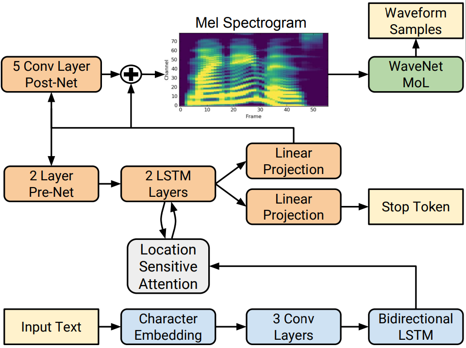
The Tacotron 2 model is a recurrent sequence-to-sequence model with attention that predicts mel-spectrograms from text. The encoder (blue blocks in the figure below) transforms the whole text into a fixed-size hidden feature representation. This feature representation is then consumed by the autoregressive decoder (orange blocks) that produces one spectrogram frame at a time. In our implementation, the autoregressive WaveNet (green block) is replaced by the flow-based generative WaveGlow.

Figure 1. Architecture of the Tacotron 2 model. Taken from the Tacotron 2 paper.

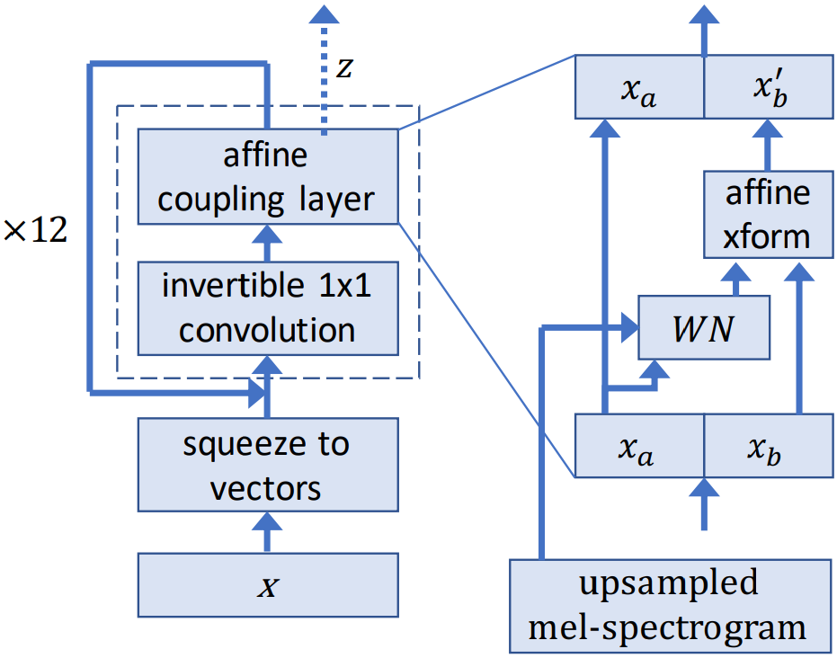
The WaveGlow model is a flow-based generative model that generates audio samples from Gaussian distribution using mel-spectrogram conditioning (Figure 2). During training, the model learns to transform the dataset distribution into spherical Gaussian distribution through a series of flows. One step of a flow consists of an invertible convolution, followed by a modified WaveNet architecture that serves as an affine coupling layer. During inference, the network is inverted and audio samples are generated from the Gaussian distribution.

Figure 2. Architecture of the WaveGlow model. Taken from the WaveGlow paper.

Default configuration

Both models support multi-GPU and mixed precision training with dynamic loss scaling (see Apex code here), as well as mixed precision inference. To speed up Tacotron 2 training, reference mel-spectrograms are generated during a preprocessing step and read directly from disk during training, instead of being generated during training.

The following features were implemented in this model:

• data-parallel multi-GPU training
• dynamic loss scaling with backoff for Tensor Cores (mixed precision) training.

Feature support matrix

The following features are supported by this model.

Feature	Tacotron 2	and WaveGlow
AMP	Yes	Yes
Apex DistributedDataParallel	Yes	Yes

Features

AMP - a tool that enables Tensor Core-accelerated training. Please refer to section Enabling mixed precision for more details.

Apex DistributedDataParallel - a module wrapper that enables easy multiprocess distributed data parallel training, similar to torch.nn.parallel.DistributedDataParallel. DistributedDataParallel is optimized for use with NCCL. It achieves high performance by overlapping communication with computation during backward() and bucketing smaller gradient transfers to reduce the total number of transfers required.

Setup

The following section lists the requirements in order to start training the Tacotron 2 and WaveGlow models.

Requirements

This repository contains Dockerfile which extends the PyTorch NGC container and encapsulates some dependencies. Aside from these dependencies, ensure you have the following components:

• NVIDIA Docker
• PyTorch 19.04-py3 NGC container or newer
• NVIDIA Volta or Turing based GPU

For more information about how to get started with NGC containers, see the following sections from the NVIDIA GPU Cloud Documentation and the Deep Learning Documentation:

• Getting Started Using NVIDIA GPU Cloud
• Accessing And Pulling From The NGC Container Registry
• Running PyTorch

For those unable to use the PyTorch NGC container, to set up the required environment or create your own container, see the versioned NVIDIA Container Support Matrix.

Quick Start Guide

To train your model using mixed precision with Tensor Cores or using FP32, perform the following steps using the default parameters of the Tacrotron 2 and WaveGlow model on the LJ Speech dataset.

1. Clone the repository.

git clone https://github.com/NVIDIA/DeepLearningExamples.git
cd DeepLearningExamples/PyTorch/SpeechSynthesis/Tacotron2

2. Download and preprocess the dataset. Use the ./scripts/prepare-dataset.sh download script to automatically download and preprocess the training, validation and test datasets. To run this script, issue:

bash scripts/prepare-dataset.sh

To preprocess the datasets for Tacotron 2 training, use the ./scripts/prepare-mels.sh script:

bash scripts/prepare_mels.sh

Data is downloaded to the ./LJSpeech-1.1 directory (on the host). The ./LJSpeech-1.1 directory is mounted to the /workspace/tacotron2/LJSpeech-1.1 location in the NGC container. The preprocessed mel-spectrograms are stored in the ./LJSpeech-1.1/mels directory.

3. Build the Tacotron 2 and WaveGlow PyTorch NGC container.

bash scripts/docker/build.sh

4. Start an interactive session in the NGC container to run training/inference. After you build the container image, you can start an interactive CLI session with:

bash scripts/docker/interactive.sh

The interactive.sh script requires that the location on the dataset is specified. For example, LJSpeech-1.1.

5. Start training. To start Tacotron 2 training, run:

bash scripts/train_tacotron2.sh

To start WaveGlow training, run:

bash scripts/train_waveglow.sh

6. Start validation/evaluation. Ensure your loss values are comparable to those listed in the table in the [Results][#results] section. For both models, the loss values are stored in the ./output/nvlog.json log file.

After you have trained the Tacotron 2 model for 1500 epochs and the WaveGlow model for 800 epochs, you should get audio results similar to the samples in the ./audio folder. For details about generating audio, see the Inference process section below.

The training scripts automatically run the validation after each training epoch. The results from the validation are printed to the standard output (stdout) and saved to the log files.

7. Start inference. After you have trained the Tacotron 2 and WaveGlow models, you can perform inference using the respective checkpoints that are passed as --tacotron2 and --waveglow arguments.

To run inference issue:

python inference.py --tacotron2 <Tacotron2_checkpoint> --waveglow <WaveGlow_checkpoint> -o output/ -i text.txt --fp16-run

The speech is generated from a text file that is passed with -i argument. To run inference in mixed precision, use the --amp-run flag. The output audio will be stored in the path specified by the -o argument.

Details

The following sections provide greater details of the dataset, running training and inference, and the training results.

Scripts and sample code

The sample code for Tacotron 2 and WaveGlow has scripts specific to a particular model, located in directories ./tacotron2 and ./waveglow, as well as scripts common to both models, located in the ./common directory. The model-specific scripts are as follows:

• <model_name>/model.py - the model architecture, definition of forward and inference functions
• <model_name>/arg_parser.py - argument parser for parameters specific to a given model
• <model_name>/data_function.py - data loading functions
• <model_name>/loss_function.py - loss function for the model

The common scripts contain layer definitions common to both models (common/layers.py), some utility scripts (common/utils.py) and scripts for audio processing (common/audio_processing.py and common/stft.py). In the root directory ./ of this repository, the ./run.py script is used for training while inference can be executed with the ./inference.py script. The scripts ./models.py, ./data_functions.py and ./loss_functions.py call the respective scripts in the <model_name> directory, depending on what model is trained using the run.py script.

Parameters

In this section, we list the most important hyperparameters and command-line arguments, together with their default values that are used to train Tacotron 2 and WaveGlow models.

Shared parameters

• --epochs - number of epochs (Tacotron 2: 1500, WaveGlow: 1000)
• --learning-rate - learning rate (Tacotron 2: 1e-3, WaveGlow: 1e-4)
• --batch-size - batch size (Tacotron 2 FP16/FP32: 80/48, WaveGlow FP16/FP32: 8/4)
• --amp-run - use mixed precision training

Shared audio/STFT parameters

• --sampling-rate - sampling rate in Hz of input and output audio (22050)
• --filter-length - (1024)
• --hop-length - hop length for FFT, i.e., sample stride between consecutive FFTs (256)
• --win-length - window size for FFT (1024)
• --mel-fmin - lowest frequency in Hz (0.0)
• --mel-fmax - highest frequency in Hz (8.000)

Tacotron 2 parameters

• --anneal-steps - epochs at which to anneal the learning rate (500 1000 1500)
• --anneal-factor - factor by which to anneal the learning rate (FP16/FP32: 0.3/0.1)

WaveGlow parameters

• --segment-length - segment length of input audio processed by the neural network (8000)

Command-line options

To see the full list of available options and their descriptions, use the -h or --help command line option, for example:

python train.py --help

Getting the data

The Tacotron 2 and WaveGlow models were trained on the LJSpeech-1.1 dataset.
This repository contains the ./scripts/prepare_dataset.sh script which will automatically download and extract the whole dataset. By default, data will be extracted to the ./LJSpeech-1.1 directory. The dataset directory contains a README file, a wavs directory with all audio samples, and a file metadata.csv that contains audio file names and the corresponding transcripts.

Dataset guidelines

The LJSpeech dataset has 13,100 clips that amount to about 24 hours of speech. Since the original dataset has all transcripts in the metadata.csv file, in this repository we provide file lists in the ./filelists directory that determine training and validation subsets; ljs_audio_text_train_filelist.txt is a test set used as a training dataset and ljs_audio_text_val_filelist.txt is a test set used as a validation dataset.

Multi-dataset

To use datasets different than the default LJSpeech dataset:

1. Prepare a directory with all audio files and pass it to the --dataset-path command-line option.

2. Add two text files containing file lists: one for the training subset (--training-files) and one for the validation subset (--validation files). The structure of the filelists should be as follows:

`<audio file path>|<transcript>`

The <audio file path> is the relative path to the path provided by the --dataset-path option.

Training process

The Tacotron2 and WaveGlow models are trained separately and independently. Both models obtain mel-spectrograms from short time Fourier transform (STFT) during training. These mel-spectrograms are used for loss computation in case of Tacotron 2 and as conditioning input to the network in case of WaveGlow.

The training loss is averaged over an entire training epoch, whereas the validation loss is averaged over the validation dataset. Performance is reported in total input tokens per second for the Tacotron 2 model and in total output samples per second for the WaveGlow model. Both measures are recorded as train_iter_items/sec (after each iteration) and train_epoch_items/sec (averaged over epoch) in the output log file ./output/nvlog.json. The result is averaged over an entire training epoch and summed over all GPUs that were included in the training.

Even though the training script uses all available GPUs, you can change this behavior by setting the CUDA_VISIBLE_DEVICES variable in your environment or by setting the NV_GPU variable at the Docker container launch (see section "GPU isolation").

Inference process

You can run inference using the ./inference.py script. This script takes text as input and runs Tacotron 2 and then WaveGlow inference to produce an audio file. It requires pre-trained checkpoints from Tacotron 2 and WaveGlow models and input text as a text file, with one phrase per line.

To run inference, issue:

python inference.py --tacotron2 <Tacotron2_checkpoint> --waveglow <WaveGlow_checkpoint> -o output/ -i text.txt --amp-run

Here, Tacotron2_checkpoint and WaveGlow_checkpoint are pre-trained checkpoints for the respective models, and text.txt contains input phrases. Audio will be saved in the output folder.

You can find all the available options by calling python inference.py --help.

Mixed precision training

Mixed precision is the combined use of different numerical precisions in a computational method. Mixed precision training offers significant computational speedup by performing operations in half-precision format, while storing minimal information in single-precision to retain as much information as possible in critical parts of the network. Since the introduction of Tensor Cores in the Volta and Turing architecture, significant training speedups are experienced by switching to mixed precision -- up to 3x overall speedup on the most arithmetically intense model architectures. Using mixed precision training requires two steps:

1. Porting the model to use the FP16 data type where appropriate.
2. Adding loss scaling to preserve small gradient values.

The ability to train deep learning networks with lower precision was introduced in the Pascal architecture and first supported in CUDA 8 in the NVIDIA Deep Learning SDK.

For information about:

• How to train using mixed precision, see the Mixed Precision Training paper and Training With Mixed Precision documentation.
• Techniques used for mixed precision training, see the Mixed-Precision Training of Deep Neural Networks blog.
• How to access and enable AMP for TensorFlow, see Using TF-AMP from the TensorFlow User Guide.
• APEX tools for mixed precision training, see the NVIDIA Apex: Tools for Easy Mixed-Precision Training in PyTorch.

Enabling mixed precision

Mixed precision is enabled in PyTorch by using the Automatic Mixed Precision (AMP) library from APEX that casts variables to half-precision upon retrieval, while storing variables in single-precision format. Furthermore, to preserve small gradient magnitudes in backpropagation, a loss scaling step must be included when applying gradients. In PyTorch, loss scaling can be easily applied by using the scale_loss() method provided by AMP. The scaling value to be used can be dynamic or fixed.

By default, the train_tacotron2.sh and train_waveglow.sh scripts will launch mixed precision training with Tensor Cores. You can change this behaviour by removing the --amp-run flag from the train.py script.

To enable mixed precision, the following steps were performed in the Tacotron 2 and WaveGlow models:

• Import AMP from APEX:

  from apex import amp
  amp.lists.functional_overrides.FP32_FUNCS.remove('softmax')
  amp.lists.functional_overrides.FP16_FUNCS.append('softmax')
  

• Initialize AMP:

  model, optimizer = amp.initialize(model, optimizer, opt_level="O1")
  

• If running on multi-GPU, wrap the model with DistributedDataParallel:

  from apex.parallel import DistributedDataParallel as DDP
  model = DDP(model)
  

• Scale loss before backpropagation (assuming loss is stored in a variable called losses)

  • Default backpropagate for FP32:

    losses.backward()
    

  • Scale loss and backpropagate with AMP:

    with optimizer.scale_loss(losses) as scaled_losses:
        scaled_losses.backward()
    

Benchmarking

The following section shows how to run benchmarks measuring the model performance in training and inference mode.

Training performance benchmark

To benchmark the training performance on a specific batch size, run:

Tacotron 2

• For 1 GPU

  • FP32

    python train.py -m Tacotron2 -o <output_dir> -lr 1e-3 --epochs 10 -bs <batch_size> --weight-decay 1e-6 --grad-clip-thresh 1.0 --cudnn-benchmark=True --log-file nvlog.json --training-files filelists/ljs_audio_text_train_subset_2500_filelist.txt --dataset-path <dataset-path>
    

  • FP16

    python train.py -m Tacotron2 -o <output_dir> -lr 1e-3 --epochs 10 -bs <batch_size> --weight-decay 1e-6 --grad-clip-thresh 1.0 --cudnn-benchmark=True --log-file nvlog.json --training-files filelists/ljs_audio_text_train_subset_2500_filelist.txt --dataset-path <dataset-path> --amp-run
    

• For multiple GPUs

  • FP32

    python -m multiproc train.py -m Tacotron2 -o <output_dir> -lr 1e-3 --epochs 10 -bs <batch_size> --weight-decay 1e-6 --grad-clip-thresh 1.0 --cudnn-benchmark=True --log-file nvlog.json --training-files filelists/ljs_audio_text_train_subset_2500_filelist.txt --dataset-path <dataset-path>
    

  • FP16

    python -m multiproc train.py -m Tacotron2 -o <output_dir> -lr 1e-3 --epochs 10 -bs <batch_size> --weight-decay 1e-6 --grad-clip-thresh 1.0 --cudnn-benchmark=True --log-file nvlog.json --training-files filelists/ljs_audio_text_train_subset_2500_filelist.txt --dataset-path <dataset-path> --amp-run
    

WaveGlow

• For 1 GPU

  • FP32

    python train.py -m WaveGlow -o <output_dir> -lr 1e-4 --epochs 10 -bs <batch_size> --segment-length  8000 --weight-decay 0 --grad-clip-thresh 3.4028234663852886e+38 --cudnn-benchmark=True --log-file nvlog.json --training-files filelists/ljs_audio_text_train_subset_1250_filelist.txt --dataset-path <dataset-path>
    

  • FP16

    python train.py -m WaveGlow -o <output_dir> -lr 1e-4 --epochs 10 -bs <batch_size> --segment-length 8000 --weight-decay 0 --grad-clip-thresh 65504.0 --cudnn-benchmark=True --log-file nvlog.json --training-files filelists/ljs_audio_text_train_subset_1250_filelist.txt --dataset-path <dataset-path> --amp-run
    

• For multiple GPUs

  • FP32

    python -m multiproc train.py -m WaveGlow -o <output_dir> -lr 1e-4 --epochs 10 -bs <batch_size> --segment-length 8000 --weight-decay 0 --grad-clip-thresh 3.4028234663852886e+38 --cudnn-benchmark=True --log-file nvlog.json --training-files filelists/ljs_audio_text_train_subset_1250_filelist.txt --dataset-path <dataset-path>
    

  • FP16

    python -m multiproc train.py -m WaveGlow -o <output_dir> -lr 1e-4 --epochs 10 -bs <batch_size> --segment-length 8000 --weight-decay 0 --grad-clip-thresh 65504.0 --cudnn-benchmark=True --log-file nvlog.json --training-files filelists/ljs_audio_text_train_subset_1250_filelist.txt --dataset-path <dataset-path> --amp-run
    

Each of these scripts runs for 10 epochs and for each epoch measures the average number of items per second. The performance results can be read from the nvlog.json files produced by the commands.

Inference performance benchmark

To benchmark the inference performance on a batch size=1, run:

• For FP32

  python inference.py --tacotron2 <Tacotron2_checkpoint> --waveglow <WaveGlow_checkpoint> -o output/ -i text.txt --log-file=output/nvlog_fp32.json
  

• For FP16

  python inference.py --tacotron2 <Tacotron2_checkpoint> --waveglow <WaveGlow_checkpoint> -o output/ -i text.txt --amp-run --log-file=output/nvlog_fp16.json
  

The log files contain performance numbers for Tacotron 2 model (number of input tokens per second, reported as tacotron2_items_per_sec) and for WaveGlow (number of output samples per second, reported as waveglow_items_per_sec).

Results

The following sections provide details on how we achieved our performance and accuracy in training and inference.

Training accuracy results

NVIDIA DGX-1 (8x V100 16G)

Our results were obtained by running the ./platform/train_{tacotron2,waveglow}_{FP16,FP32}_DGX1_16GB_8GPU.sh training script in the PyTorch-19.04-py3 NGC container on NVIDIA DGX-1 with 8x V100 16G GPUs.

All of the results were produced using the train.py script as described in the Training process section of this document.

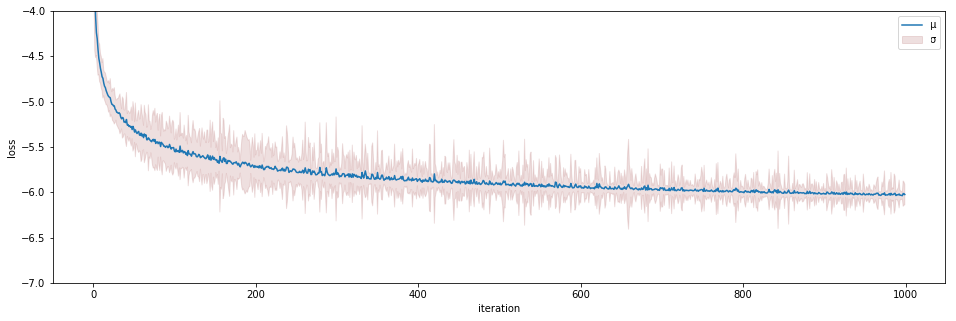
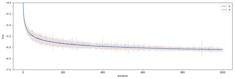
Loss (Model/Epoch)	1	250	500	750	1000
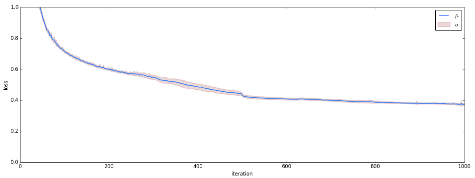
Tacotron 2 FP16	13.0732	0.5736	0.4408	0.3923	0.3735
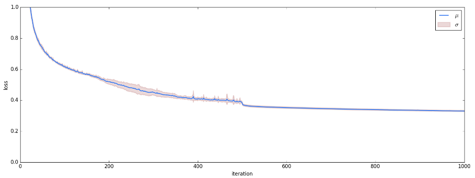
Tacotron 2 FP32	8.5776	0.4807	0.3875	0.3421	0.3308
WaveGlow FP16	-2.2054	-5.7602	-5.901	-5.9706	-6.0258
WaveGlow FP32	-3.0327	-5.858	-6.0056	-6.0613	-6.1087

Tacotron 2 FP16 loss - batch size 80 (mean and std over 16 runs)

Tacotron 2 FP32 loss - batch size 48 (mean and std over 16 runs)

WaveGlow FP16 loss - batch size 8 (mean and std over 16 runs)

WaveGlow FP32 loss - batch size 4 (mean and std over 16 runs)

Training performance results

NVIDIA DGX-1 (8x V100 16G)

Our results were obtained by running the ./platform/train_{tacotron2,waveglow}_{FP16,FP32}_DGX1_16GB_8GPU.sh training script in the PyTorch-19.04-py3 NGC container on NVIDIA DGX-1 with 8x V100 16G GPUs. Performance numbers (in input tokens per second for Tacotron 2 and output samples per second for WaveGlow) were averaged over an entire training epoch.

This table shows the results for Tacotron 2:

Number of GPUs	Batch size per GPU	Number of tokens used with mixed precision	Number of tokens used with FP32	Speed-up with mixed precision	Multi-GPU weak scaling with mixed precision	Multi-GPU weak scaling with FP32
1	128@FP16, 64@FP32	3,746	2,087	1.79	1.00	1.00
4	128@FP16, 64@FP32	13,264	8,052	1.65	3.54	3.86
8	128@FP16, 64@FP32	25,056	15,863	1.58	6.69	7.60

The following table shows the results for WaveGlow:

Number of GPUs	Batch size per GPU	Number of samples used with mixed precision	Number of samples used with FP32	Speed-up with mixed precision	Multi-GPU weak scaling with mixed precision	Multi-GPU weak scaling with FP32
1	10@FP16, 4@FP32	79248.87426	35695.56774	2.22	1.00	1.00
4	10@FP16, 4@FP32	275310.0262	126497.6265	2.18	3.47	3.54
8	10@FP16, 4@FP32	576709.4935	255155.1798	2.26	7.28	7.15

To achieve these same results, follow the steps in the Quick Start Guide.

Expected training time

The following table shows the expected training time for convergence for Tacotron 2 (1500 epochs):

|Number of GPUs|Batch size per GPU|Time to train with mixed precision (Hrs)|Time to train with FP32 (Hrs)|Speed-up with mixed precision| |---:|---:|---:|---:| |1| 128@FP16, 64@FP32 | 137.33 | 227.66 | 1.66 | |4| 128@FP16, 64@FP32 | 40.68 | 63.99 | 1.57 | |8| 128@FP16, 64@FP32 | 20.74 | 32.47 | 1.57 |

The following table shows the expected training time for convergence for WaveGlow (1000 epochs):

|Number of GPUs|Batch size per GPU|Time to train with mixed precision (Hrs)|Time to train with FP32 (Hrs)|Speed-up with mixed precision| |---:|---:|---:|---:| |1| 10@FP16, 4@FP32 | 358.00 | 793.97 | 2.22 | |4| 10@FP16, 4@FP32 | 103.10 | 223.59 | 2.17 | |8| 10@FP16, 4@FP32 | 50.40 | 109.45 | 2.17 |

Inference performance results

NVIDIA DGX-1 (8x V100 16G)

Our results were obtained by running the ./inference.py inference script in the PyTorch-18.12.1-py3 NGC container on NVIDIA DGX-1 with 8x V100 16G GPUs. Performance numbers (in input tokens per second for Tacotron 2 and output samples per second for WaveGlow) were averaged over 16 runs.

The following table shows the inference performance results for Tacotron 2. Results are measured in the number of input tokens per second.

Number of GPUs	Number of tokens used with mixed precision	Number of tokens used with FP32	Speed-up with mixed precision
1	168	173	0.97

The following table shows the inference performance results for WaveGlow. Results are measured in the number of output audio samples per second.¹

Number of GPUs	Number of samples used with mixed precision	Number of samples used with FP32	Speed-up with mixed precision
1	583318	553380	1.05

¹With sampling rate equal to 22050, one second of audio is generated from 22050 samples.

To achieve these same results, follow the steps in the Quick Start Guide.

Changelog

March 2019

• Initial release

June 2019

• AMP support
• Data preprocessing for Tacotron 2 training
• Fixed dropouts on LSTMCells

Known issues

There are no known issues in this release.