DeepLearningExamples/PyTorch/Detection/SSD/README.md

SSD300 v1.1 For PyTorch

This repository provides a script and recipe to train the SSD300 v1.1 model to achieve state of the art accuracy, and is tested and maintained by NVIDIA.

Table Of Contents

• Model overview
  • Model architecture
  • Default configuration
  • Feature support matrix
    • Features
  • Mixed precision training
    • Enabling mixed precision
    • Enabling TF32
• Setup
  • Requirements
• Quick Start Guide
• Advanced
  • Scripts and sample code
  • Parameters
  • Command-line options
  • Getting the data
    • Dataset guidelines
      • Data preprocessing
      • Data augmentation
  • Training process
  • Evaluation process
  • Inference process
• Performance
  • Benchmarking
    • Training performance benchmark
    • Inference performance benchmark
  • Results
    • Training accuracy results
      • Training accuracy: NVIDIA DGX A100 (8x A100 40GB)
      • Training accuracy: NVIDIA DGX-1 (8x V100 16GB)
      • Training loss plot
      • Training stability test
    • Training performance results
      • Training performance: NVIDIA DGX A100 (8x A100 40GB)
      • Training performance: NVIDIA DGX-1 (8x V100 16G)
    • Inference performance results
      • Inference performance: NVIDIA DGX A100 (1x A100 40GB)
      • Inference performance: NVIDIA DGX-1 (1x V100 16GB)
• Release notes
  • Changelog
  • Known issues

Model overview

The SSD300 v1.1 model is based on the SSD: Single Shot MultiBox Detector paper, which describes SSD as “a method for detecting objects in images using a single deep neural network". The input size is fixed to 300x300.

The main difference between this model and the one described in the paper is in the backbone. Specifically, the VGG model is obsolete and is replaced by the ResNet-50 model.

From the Speed/accuracy trade-offs for modern convolutional object detectors paper, the following enhancements were made to the backbone:

• The conv5_x, avgpool, fc and softmax layers were removed from the original classification model.
• All strides in conv4_x are set to 1x1.

Detector heads are similar to the ones referenced in the paper, however, they are enhanced by additional BatchNorm layers after each convolution.

Additionally, we removed weight decay on every bias parameter and all the BatchNorm layer parameters as described in the Highly Scalable Deep Learning Training System with Mixed-Precision: Training ImageNet in Four Minutes paper.

Training of SSD requires computational costly augmentations. To fully utilize GPUs during training we are using the NVIDIA DALI library to accelerate data preparation pipelines.

This model is trained with mixed precision using Tensor Cores on Volta, Turing, and the NVIDIA Ampere GPU architectures. Therefore, researchers can get results 2x faster than training without Tensor Cores, while experiencing the benefits of mixed precision training. This model is tested against each NGC monthly container release to ensure consistent accuracy and performance over time.

Model architecture

Despite the changes described in the previous section, the overall architecture, as described in the following diagram, has not changed.

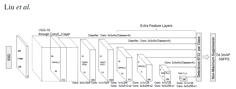
Figure 1. The architecture of a Single Shot MultiBox Detector model. Image has been taken from the Single Shot MultiBox Detector paper.

The backbone is followed by 5 additional convolutional layers. In addition to the convolutional layers, we attached 6 detection heads:

• The first detection head is attached to the last conv4_x layer.
• The other five detection heads are attached to the corresponding 5 additional layers.

Default configuration

We trained the model for 65 epochs with the following setup:

• SGD with momentum (0.9)
• Learning rate = 2.6e-3 * number of GPUs * (batch_size / 32)
• Learning rate decay – multiply by 0.1 before 43 and 54 epochs
• We use linear warmup of the learning rate during the first epoch.

For more information, see the Accurate, Large Minibatch SGD: Training ImageNet in 1 Hour paper.

To enable warmup provide argument the --warmup 300

• Weight decay: * 0 for BatchNorms and biases * 5e-4 for other layers

Note: The learning rate is automatically scaled (in other words, multiplied by the number of GPUs and multiplied by the batch size divided by 32).

Feature support matrix

The following features are supported by this model.

Feature	SSD300 v1.1 PyTorch
APEX AMP	Yes
APEX DDP	Yes
NVIDIA DALI	Yes

Features

APEX is a PyTorch extension with NVIDIA-maintained utilities to streamline mixed precision and distributed training, whereas AMP is an abbreviation used for automatic mixed precision training.

DDP stands for DistributedDataParallel and is used for multi-GPU training.

NVIDIA DALI - DALI is a library accelerating data preparation pipeline. To accelerate your input pipeline, you only need to define your data loader with the DALI library. For details, see example sources in this repo or see the DALI documentation

Mixed precision training

Mixed precision is the combined use of different numerical precisions in a computational method. Mixed precision training offers significant computational speedup by performing operations in half-precision format, while storing minimal information in single-precision to retain as much information as possible in critical parts of the network. Since the introduction of Tensor Cores in Volta, and following with both the Turing and Ampere architectures, significant training speedups are experienced by switching to mixed precision -- up to 3x overall speedup on the most arithmetically intense model architectures. Using mixed precision training requires two steps:

1. Porting the model to use the FP16 data type where appropriate.
2. Adding loss scaling to preserve small gradient values.

The ability to train deep learning networks with lower precision was introduced in the Pascal architecture and first supported in CUDA 8 in the NVIDIA Deep Learning SDK.

For information about:

• How to train using mixed precision, see the Mixed Precision Training paper and Training With Mixed Precision documentation.
• Techniques used for mixed precision training, see the Mixed-Precision Training of Deep Neural Networks blog.
• APEX tools for mixed precision training, see the NVIDIA Apex: Tools for Easy Mixed-Precision Training in PyTorch.

Enabling mixed precision

Mixed precision is enabled in PyTorch by using the Automatic Mixed Precision (AMP) library from APEX which casts variables to half-precision upon retrieval, while storing variables in single-precision format. Furthermore, to preserve small gradient magnitudes in backpropagation, a loss scaling step must be included when applying gradients. In PyTorch, loss scaling can be easily applied by using scale_loss() method provided by AMP. The scaling value to be used can be dynamic or fixed.

For an in-depth walk through on AMP, check out sample usage here. APEX is a PyTorch extension that contains utility libraries, such as AMP, which require minimal network code changes to leverage Tensor Cores performance.

To enable mixed precision, you can:

• Import AMP from APEX:

  from apex import amp
  

• Initialize an AMP handle:

  amp_handle = amp.init(enabled=True, verbose=True)
  

• Wrap your optimizer with the AMP handle:

  optimizer = amp_handle.wrap_optimizer(optimizer)
  

• Scale loss before backpropagation (assuming loss is stored in a variable called losses)

  • Default backpropagate for FP32/TF32:

    losses.backward()
    

  • Scale loss and backpropagate with AMP:

    with optimizer.scale_loss(losses) as scaled_losses:
       scaled_losses.backward()
    

Enabling TF32

TensorFloat-32 (TF32) is the new math mode in NVIDIA A100 GPUs for handling the matrix math also called tensor operations. TF32 running on Tensor Cores in A100 GPUs can provide up to 10x speedups compared to single-precision floating-point math (FP32) on Volta GPUs.

TF32 Tensor Cores can speed up networks using FP32, typically with no loss of accuracy. It is more robust than FP16 for models which require high dynamic range for weights or activations.

For more information, refer to the TensorFloat-32 in the A100 GPU Accelerates AI Training, HPC up to 20x blog post.

TF32 is supported in the NVIDIA Ampere GPU architecture and is enabled by default.

Glossary

backbone

a part of a many object detection architectures, usually pre-trained for a different, simpler task, like classification.

input pipeline

set of operations performed for every item in input data before feeding the neural network. Especially for object detection task, the input pipeline can be complex and computationally significant. For that reason, solutions like NVIDIA DALI emerged.

object detection

a subset of Computer Vision problem. The task of object detection is to localize possibly multiple objects on the image and classify them. The difference between Object Detection, Image Classification, and Localization are clearly explained in the video published as a part of the C4W3L01 course.

SSD (Single Shot MultiBox Detector)

a name for the detection model described in a paper authored by Liu at al.

ResNet (ResNet-50)

a name for the classification model described in a paper authored by He et al. In this repo, it is used as a backbone for SSD.

Setup

The following section lists the requirements in order to start training the SSD300 v1.1 model.

Requirements

This repository contains Dockerfile which extends the PyTorch 20.06 NGC container and encapsulates some dependencies. Aside from these dependencies, ensure you have the following software:

• NVIDIA Docker
• PyTorch 20.06-py3+ NGC container
• GPU-based architecture:
  • NVIDIA Volta
  • NVIDIA Turing
  • NVIDIA Ampere architecture

For more information about how to get started with NGC containers, see the following sections from the NVIDIA GPU Cloud Documentation and the Deep Learning Documentation:

• Getting Started Using NVIDIA GPU Cloud
• Accessing And Pulling From The NGC Container Registry
• Running PyTorch

For those unable to use the PyTorch 20.06-py3 NGC container, to set up the required environment or create your own container, see the versioned NVIDIA Container Support Matrix.

Quick Start Guide

To train your model using mixed or TF32 precision with Tensor Cores or using FP32, perform the following steps using the default parameters of the SSD v1.1 model on the COCO 2017 dataset. For the specifics concerning training and inference, see the Advanced section.

1. Clone the repository.

git clone https://github.com/NVIDIA/DeepLearningExamples
cd DeepLearningExamples/PyTorch/Detection/SSD

2. Download and preprocess the dataset.

Extract the COCO 2017 dataset with download_dataset.sh $COCO_DIR. Data will be downloaded to the $COCO_DIR directory (on the host).

3. Build the SSD300 v1.1 PyTorch NGC container.

docker build . -t nvidia_ssd

4. Start an interactive session in the NGC container to run training/inference.

nvidia-docker run --rm -it --ulimit memlock=-1 --ulimit stack=67108864 -v $COCO_DIR:/coco --ipc=host nvidia_ssd

Note: the default mount point in the container is /coco.

5. Start training.

The ./examples directory provides several sample scripts for various GPU settings and act as wrappers around the main.py script. The example scripts need two arguments:

• A path to the root SSD directory.
• A path to the COCO 2017 dataset.

Remaining arguments are passed to the main.py script.

The --save save_dir flag, saves the model after each epoch in save_dir directory. The checkpoints are stored as <save_dir>/epoch_*.pt.

Use python main.py -h to obtain the list of available options in the main.py script. For example, if you want to run 8 GPU training with Tensor Core acceleration and save checkpoints after each epoch, run:

bash ./examples/SSD300_FP16_8GPU.sh . /coco --save

6. Start validation/evaluation.

The main.py training script automatically runs validation during training. The results from the validation are printed to stdout.

To evaluate a checkpointed model saved in the previous point, run:

python ./main.py --backbone resnet50 --mode evaluation --checkpoint ./models/epoch_*.pt --data /coco

7. Optionally, resume training from a checkpointed model.

python ./main.py --backbone resnet50 --checkpoint ./models/epoch_*.pt --data /coco

8. Start inference/predictions.

You can check your trained model with a Jupyter notebook provided in the examples directory. Start with running a Docker container with a Jupyter notebook server:

nvidia-docker run --rm -it --ulimit memlock=-1 --ulimit stack=67108864 -v $SSD_CHECKPINT_PATH:/checkpoints/SSD300v1.1.pt -v $COCO_PATH:/datasets/coco2017 --ipc=host -p 8888:8888 nvidia_ssd jupyter-notebook --ip 0.0.0.0 --allow-root

Advanced

The following sections provide greater details of the dataset, running training and inference, and the training results.

Scripts and sample code

In the root directory, the most important files are:

• main.py: the script that controls the logic of training and validation of the SSD300 v1.1 model;
• Dockerfile: Instructions for docker to build a container with the basic set of dependencies to run SSD300 v1.1;
• requirements.txt: a set of extra Python requirements for running SSD300 v1.1;
• download_dataset.py: automatically downloads the COCO dataset for training.

The src/ directory contains modules used to train and evaluate the SSD300 v1.1 model

• model.py: the definition of SSD300 v1.1 model
• data.py: definition of input pipelines used in training and evaluation
• train.py: functions used to train the SSD300 v1.1 model
• evaluate.py: functions used to evaluate the SSD300 v1.1 model
• coco_pipeline.py: definition of input pipeline using NVIDIA DALI
• coco.py: code specific for the COCO dataset
• logger.py: utilities for logging
• utils.py: extra utility functions

The examples/ directory contains scripts wrapping common scenarios.

Parameters

The script main.py

The script for training end evaluating the SSD300 v1.1 model have a variety of parameters that control these processes.

Common parameters

--data

use it to specify, where your dataset is. By default, the script will look for it under the /coco directory.

--checkpoint

allows you to specify the path to the pre-trained model.

--save

when the flag is turned on, the script will save the trained model checkpoints in the specified directory

--seed

Use it to specify the seed for RNGs.

--amp

when the flag is turned on, the AMP features will be enabled.

Training related

--epochs

a number of times the model will see every example from the training dataset.

--evaluation

after this parameter, list the number of epochs after which evaluation should be performed.

--learning-rate

initial learning rate.

--multistep

after this parameter, list the epochs after which learning rate should be decayed.

--warmup

allows you to specify the number of iterations for which a linear learning-rate warmup will be performed.

--momentum

momentum argument for SGD optimizer.

--weight-decay

weight decay argument for SGD optimizer.

--batch-size

a number of inputs processed at once for each iteration.

--backbone-path

the path to the checkpointed backbone. When it is not provided, a pre-trained model from torchvision will be downloaded.

Evaluation related

--eval-batch-size

a number of inputs processed at once for each iteration.

Utility parameters

--help

displays a short description of all parameters accepted by the script.

Command-line options

All these parameters can be controlled by passing command-line arguments to the main.py script. To get a complete list of all command-line arguments with descriptions and default values you can run:

python main.py --help

Getting the data

The SSD model was trained on the COCO 2017 dataset. The val2017 validation set was used as a validation dataset. PyTorch can work directly on JPEGs, therefore, preprocessing/augmentation is not needed.

This repository contains the download_dataset.sh download script which will automatically download and preprocess the training, validation and test datasets. By default, data will be downloaded to the /coco directory.

Dataset guidelines

Our model expects input data aligned in a way a COCO dataset is aligned by the download_dataset.sh script. train2017 and val2017 directories should contain images in JPEG format. Annotation format is described in the COCO documentation.

The preprocessing of the data is defined in the src/coco_pipeline.py module.

Data preprocessing

Before we feed data to the model, both during training and inference, we perform:

• JPEG decoding
• normalization with a mean = [0.485, 0.456, 0.406] and std dev = [0.229, 0.224, 0.225]
• encoding bounding boxes
• resizing to 300x300

Additionally, during training, data is:

• randomly shuffled
• samples without annotations are skipped

Data augmentation

During training we perform the following augmentation techniques:

• Random crop using the algorithm described in the SSD: Single Shot MultiBox Detector paper
• Random horizontal flip
• Color jitter

Training process

Training the SSD model is implemented in the main.py script.

By default, training is running for 65 epochs. Because evaluation is relatively time consuming, it is not running every epoch. With default settings, evaluation is executed after epochs: 21, 31, 37, 42, 48, 53, 59, 64. The model is evaluated using pycocotools distributed with the COCO dataset. Which epochs should be evaluated can be reconfigured with the --evaluation argument.

To run training with Tensor Cores, use the --amp flag when running the main.py script. The flag --save ./models flag enables storing checkpoints after each epoch under ./models/epoch_*.pt.

Evaluation process

Pycocotools’ open-sourced scripts provides a consistent way to evaluate models on the COCO dataset. We are using these scripts during validation to measure a models performance in AP metric. Metrics below are evaluated using pycocotools’ methodology, in the following format:

 Average Precision  (AP) @[ IoU=0.50:0.95 | area=   all | maxDets=100 ] = 0.250
 Average Precision  (AP) @[ IoU=0.50      | area=   all | maxDets=100 ] = 0.423
 Average Precision  (AP) @[ IoU=0.75      | area=   all | maxDets=100 ] = 0.257
 Average Precision  (AP) @[ IoU=0.50:0.95 | area= small | maxDets=100 ] = 0.076
 Average Precision  (AP) @[ IoU=0.50:0.95 | area=medium | maxDets=100 ] = 0.269
 Average Precision  (AP) @[ IoU=0.50:0.95 | area= large | maxDets=100 ] = 0.399
 Average Recall     (AR) @[ IoU=0.50:0.95 | area=   all | maxDets=  1 ] = 0.237
 Average Recall     (AR) @[ IoU=0.50:0.95 | area=   all | maxDets= 10 ] = 0.342
 Average Recall     (AR) @[ IoU=0.50:0.95 | area=   all | maxDets=100 ] = 0.358
 Average Recall     (AR) @[ IoU=0.50:0.95 | area= small | maxDets=100 ] = 0.118
 Average Recall     (AR) @[ IoU=0.50:0.95 | area=medium | maxDets=100 ] = 0.394
 Average Recall     (AR) @[ IoU=0.50:0.95 | area= large | maxDets=100 ] = 0.548

The metric reported in our results is present in the first row.

Inference process

Our scripts for SSD300 v1.1 presents two ways to run inference. To get meaningful results, you need a pre-trained model checkpoint.

One way is to run an interactive session on Jupyter notebook, as described in a 8th step of the Quick Start Guide.

The container prints Jupyter notebook logs like this:

[I 16:17:58.935 NotebookApp] Writing notebook server cookie secret to /root/.local/share/jupyter/runtime/notebook_cookie_secret
[I 16:17:59.769 NotebookApp] JupyterLab extension loaded from /opt/conda/lib/python3.6/site-packages/jupyterlab
[I 16:17:59.769 NotebookApp] JupyterLab application directory is /opt/conda/share/jupyter/lab
[I 16:17:59.770 NotebookApp] Serving notebooks from local directory: /workspace
[I 16:17:59.770 NotebookApp] The Jupyter Notebook is running at: 
[I 16:17:59.770 NotebookApp] http://(65935d756c71 or 127.0.0.1):8888/?token=04c78049c67f45a4d759c8f6ddd0b2c28ac4eab60d81be4e
[I 16:17:59.770 NotebookApp] Use Control-C to stop this server and shut down all kernels (twice to skip confirmation).
[W 16:17:59.774 NotebookApp] No web browser found: could not locate runnable browser.
[C 16:17:59.774 NotebookApp] 
        
    To access the notebook, open this file in a browser:
        file:///root/.local/share/jupyter/runtime/nbserver-1-open.html
    Or copy and paste one of these URLs:
        http://(65935d756c71 or 127.0.0.1):8888/?token=04c78049c67f45a4d759c8f6ddd0b2c28ac4eab60d81be4e

Use the token printed in the last line to start your notebook session. The notebook is in examples/inference.ipynb, for example:

http://127.0.0.1:8888/notebooks/examples/inference.ipynb?token=04c78049c67f45a4d759c8f6ddd0b2c28ac4eab60d81be4e

Another way is to run a script examples/SSD300_inference.py. It contains the logic from the notebook, wrapped into a Python script. The script contains sample usage.

To use the inference example script in your own code, you can call the main function, providing input image URIs as an argument. The result will be a list of detections for each input image.

Performance

The performance measurements in this document were conducted at the time of publication and may not reflect the performance achieved from NVIDIA’s latest software release. For the most up-to-date performance measurements, go to NVIDIA Data Center Deep Learning Product Performance.

Benchmarking

The following section shows how to run benchmarks measuring the model performance in training and inference modes.

Training performance benchmark

The training benchmark was run in various scenarios on A100 40GB and V100 16G GPUs. The benchmark does not require a checkpoint from a fully trained model.

To benchmark training, run:

python -m torch.distributed.launch --nproc_per_node={NGPU} \
       main.py --batch-size {bs} \
               --mode benchmark-training \
               --benchmark-warmup 100 \
               --benchmark-iterations 200 \
               {AMP} \
               --data {data}

Where the {NGPU} selects number of GPUs used in benchmark, the {bs} is the desired batch size, the {AMP} is set to --amp if you want to benchmark training with Tensor Cores, and the {data} is the location of the COCO 2017 dataset.

--benchmark-warmup is specified to omit the first iteration of the first epoch. --benchmark-iterations is a number of iterations used to measure performance.

Inference performance benchmark

Inference benchmark was run on 1x A100 40GB GPU and 1x V100 16G GPU. To benchmark inference, run:

python main.py --eval-batch-size {bs} \
               --mode benchmark-inference \
               --benchmark-warmup 100 \
               --benchmark-iterations 200 \
               {AMP} \
               --data {data}

Where the {bs} is the desired batch size, the {AMP} is set to --amp if you want to benchmark inference with Tensor Cores, and the {data} is the location of the COCO 2017 dataset.

--benchmark-warmup is specified to omit the first iterations of the first epoch. --benchmark-iterations is a number of iterations used to measure performance.

Results

The following sections provide details on how we achieved our performance and accuracy in training and inference.

Training accuracy results

Training accuracy: NVIDIA DGX A100 (8x A100 40GB)

Our results were obtained by running the ./examples/SSD300_A100_{FP16,TF32}_{1,4,8}GPU.sh script in the pytorch-20.06-py3 NGC container on NVIDIA DGX A100 (8x A100 40GB) GPUs.

GPUs	Batch size / GPU	Accuracy - TF32	Accuracy - mixed precision	Time to train - TF32	Time to train - mixed precision	Time to train speedup (TF32 to mixed precision)
1	64	0.251	0.252	16:00:00	8:00:00	200.00%
4	64	0.250	0.251	3:00:00	1:36:00	187.50%
8	64	0.252	0.251	1:40:00	1:00:00	167.00%
1	128	0.251	0.251	13:05:00	7:00:00	189.05%
4	128	0.252	0.253	2:45:00	1:30:00	183.33%
8	128	0.248	0.249	1:20:00	0:43:00	186.00%

Training accuracy: NVIDIA DGX-1 (8x V100 16GB)

Our results were obtained by running the ./examples/SSD300_FP{16,32}_{1,4,8}GPU.sh script in the pytorch-20.06-py3 NGC container on NVIDIA DGX-1 with 8x V100 16GB GPUs.

GPUs	Batch size / GPU	Accuracy - FP32	Accuracy - mixed precision	Time to train - FP32	Time to train - mixed precision	Time to train speedup (FP32 to mixed precision)
1	32	0.250	0.250	20:20:13	10:23:46	195.62%
4	32	0.249	0.250	5:11:17	2:39:28	195.20%
8	32	0.250	0.250	2:37:00	1:32:00	170.60%
1	64	<N/A>	0.252	<N/A>	9:27:33	215.00%
4	64	<N/A>	0.251	<N/A>	2:24:43	215.10%
8	64	<N/A>	0.252	<N/A>	1:31:00	172.50%

Due to smaller size, mixed precision models can be trained with bigger batches. In such cases mixed precision speedup is calculated versus FP32 training with maximum batch size for that precision

Training loss plot

Here are example graphs of FP32, TF32 and AMP training on 8 GPU configuration:

Training stability test

The SSD300 v1.1 model was trained for 65 epochs, starting from 15 different initial random seeds. The training was performed in the pytorch-20.06-py3 NGC container on NVIDIA DGX A100 8x A100 40GB GPUs with batch size per GPU = 128. After training, the models were evaluated on the test dataset. The following table summarizes the final mAP on the test set.

Precision	Average mAP	Standard deviation	Minimum	Maximum	Median
AMP	0.2491314286	0.001498316675	0.24456	0.25182	0.24907
TF32	0.2489106667	0.001749463047	0.24487	0.25148	0.24848

Training performance results

Training performance: NVIDIA DGX A100 (8x A100 40GB)

Our results were obtained by running the main.py script with the --mode benchmark-training flag in the pytorch-20.06-py3 NGC container on NVIDIA DGX A100 (8x A100 40GB) GPUs. Performance numbers (in items/images per second) were averaged over an entire training epoch.

GPUs	Batch size / GPU	Throughput - TF32	Throughput - mixed precision	Throughput speedup (TF32 - mixed precision)	Weak scaling - TF32	Weak scaling - mixed precision
1	64	201.43	367.15	182.27%	100.00%	100.00%
4	64	791.50	1,444.00	182.44%	392.94%	393.30%
8	64	1,582.72	2,872.48	181.49%	785.74%	782.37%
1	128	206.28	387.95	188.07%	100.00%	100.00%
4	128	822.39	1,530.15	186.06%	398.68%	397.73%
8	128	1,647.00	3,092.00	187.74%	798.43%	773.00%

To achieve these same results, follow the Quick Start Guide outlined above.

Training performance: NVIDIA DGX-1 (8x V100 16GB)

Our results were obtained by running the main.py script with the --mode benchmark-training flag in the pytorch-20.06-py3 NGC container on NVIDIA DGX-1 with 8x V100 16GB GPUs. Performance numbers (in items/images per second) were averaged over an entire training epoch.

GPUs	Batch size / GPU	Throughput - FP32	Throughput - mixed precision	Throughput speedup (FP32 - mixed precision)	Weak scaling - FP32	Weak scaling - mixed precision
1	32	133.67	215.30	161.07%	100.00%	100.00%
4	32	532.05	828.63	155.74%	398.04%	384.88%
8	32	820.70	1,647.74	200.77%	614.02%	802.00%
1	64	<N/A>	232.22	173.73%	<N/A>	100.00%
4	64	<N/A>	910.77	171.18%	<N/A>	392.20%
8	64	<N/A>	1,728.00	210.55%	<N/A>	761.99%

Due to smaller size, mixed precision models can be trained with bigger batches. In such cases mixed precision speedup is calculated versus FP32 training with maximum batch size for that precision

To achieve these same results, follow the Quick Start Guide outlined above.

Inference performance results

Inference performance: NVIDIA DGX A100 (1x A100 40GB)

Our results were obtained by running the main.py script with --mode benchmark-inference flag in the pytorch-20.06-py3 NGC container on NVIDIA DGX A100 (1x A100 40GB) GPU.

Batch size	Throughput - TF32	Throughput - mixed precision	Throughput speedup (TF32 - mixed precision)	Weak scaling - TF32	Weak scaling - mixed precision
1	113.51	109.93	96.85%	100.00%	100.00%
2	203.07	214.43	105.59%	178.90%	195.06%
4	338.76	368.45	108.76%	298.30%	335.17%
8	485.65	526.97	108.51%	427.85%	479.37%
16	493.64	867.42	175.72%	434.89%	789.07%
32	548.75	910.17	165.86%	483.44%	827.95%

To achieve these same results, follow the Quick Start Guide outlined above.

Inference performance: NVIDIA DGX-1 (1x V100 16GB)

Our results were obtained by running the main.py script with --mode benchmark-inference flag in the pytorch-20.06-py3 NGC container on NVIDIA DGX-1 with (1x V100 16GB) GPU.

Batch size	Throughput - FP32	Throughput - mixed precision	Throughput speedup (FP32 - mixed precision)	Weak scaling - FP32	Weak scaling - mixed precision
1	82.50	80.50	97.58%	100.00%	100.00%
2	124.05	147.46	118.87%	150.36%	183.18%
4	155.51	255.16	164.08%	188.50%	316.97%
8	182.37	334.94	183.66%	221.05%	416.07%
16	222.83	358.25	160.77%	270.10%	445.03%
32	271.73	438.85	161.50%	329.37%	545.16%

To achieve these same results, follow the Quick Start Guide outlined above.

Release notes

Changelog

June 2020

• upgrade the PyTorch container to 20.06
• update performance tables to include A100 results
• update examples with A100 configs

August 2019

• upgrade the PyTorch container to 19.08
• update Results section in the README
• code updated to use DALI 0.12.0
• checkpoint loading fix
• fixed links in the README

July 2019

• script and notebook for inference
• use AMP instead of hand-crafted FP16 support
• README update
• introduced a parameter with a path to the custom backbone checkpoint
• minor enchantments of example/* scripts
• alignment to changes in PyTorch 19.06

March 2019

• Initial release

Known issues

There are no known issues with this model.