41 KiB
FastPitch 1.0 for PyTorch
This repository provides a script and recipe to train the FastPitch model to achieve state-of-the-art accuracy and is tested and maintained by NVIDIA.
Table Of Contents
Model overview
FastPitch is a fully-parallel transformer architecture with prosody control over pitch and individual phoneme duration. It is one of two major components in a neural, text-to-speech (TTS) system:
- a mel-spectrogram generator such as FastPitch or Tacotron 2, and
- a waveform synthesizer such as WaveGlow (see NVIDIA example code).
Such two-component TTS system is able to synthesize natural sounding speech from raw transcripts.
The FastPitch model generates mel-spectrograms and predicts a pitch contour from raw input text. Some of the capabilities of FastPitch are presented on the website with samples.
Speech synthesized with FastPitch has state-of-the-art quality, and does not suffer from missing/repeating phrases like Tacotron2 does. This is reflected in Mean Opinion Scores (details).
| Model | Mean Opinion Score (MOS) |
|---|---|
| Tacotron2 | 3.946 ± 0.134 |
| FastPitch | 4.080 ± 0.133 |
The FastPitch model is based on the FastSpeech model. The main differences between FastPitch and FastSpeech are that FastPitch:
- explicitly learns to predict the pitch contour,
- pitch conditioning removes harsh sounding artifacts and provides faster convergence,
- no need for distilling mel-spectrograms with a teacher model,
- character durations are extracted with a pre-trained Tacotron 2 model.
The FastPitch model is similar to FastSpeech2, which has been developed concurrently. FastPitch averages pitch values over input tokens, and does not use additional conditioning such as the energy.
FastPitch is trained on a publicly available LJ Speech dataset.
This model is trained with mixed precision using Tensor Cores on Volta, Turing, and the NVIDIA Ampere GPU architectures. Therefore, researchers can get results from 2.0x to 2.7x faster than training without Tensor Cores, while experiencing the benefits of mixed precision training. This model is tested against each NGC monthly container release to ensure consistent accuracy and performance over time.
Model architecture
FastPitch is a fully feedforward Transformer model that predicts mel-spectrograms from raw text (Figure 1). The entire process is parallel, which means that all input letters are processed simultaneously to produce a full mel-spectrogram in a single forward pass.
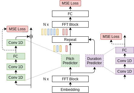
Figure 1. Architecture of FastPitch (source). The model is composed of a bidirectional Transformer backbone (also known as a Transformer encoder), a pitch predictor, and a duration predictor. After passing through the first *N* Transformer blocks, encoding, the signal is augmented with pitch information and discretely upsampled. Then it goes through another set of *N* Transformer blocks, with the goal of smoothing out the upsampled signal, and constructing a mel-spectrogram.
Default configuration
The FastPitch model supports multi-GPU and mixed precision training with dynamic loss scaling (see Apex code here), as well as mixed precision inference.
The following features were implemented in this model:
- data-parallel multi-GPU training,
- dynamic loss scaling with backoff for Tensor Cores (mixed precision) training,
- gradient accumulation for reproducible results regardless of the number of GPUs.
To speed-up FastPitch training, reference mel-spectrograms, character durations, and pitch cues are generated during the pre-processing step and read directly from the disk during training. For more information on data pre-processing refer to Dataset guidelines and the paper.
Feature support matrix
The following features are supported by this model.
| Feature | FastPitch |
|---|---|
| AMP | Yes |
| Apex DistributedDataParallel | Yes |
Features
AMP - a tool that enables Tensor Core-accelerated training. For more information, refer to Enabling mixed precision.
Apex DistributedDataParallel - a module wrapper that enables easy multiprocess
distributed data parallel training, similar to torch.nn.parallel.DistributedDataParallel.
DistributedDataParallel is optimized for use with NCCL. It achieves high
performance by overlapping communication with computation during backward()
and bucketing smaller gradient transfers to reduce the total number of transfers
required.
Mixed precision training
Mixed precision is the combined use of different numerical precisions in a computational method. Mixed precision training offers significant computational speedup by performing operations in half-precision format while storing minimal information in single-precision to retain as much information as possible in critical parts of the network. Since the introduction of Tensor Cores in Volta, and following with both the Turing and Ampere architectures, significant training speedups are experienced by switching to mixed precision -- up to 3x overall speedup on the most arithmetically intense model architectures. Using mixed precision training requires two steps:
- Porting the model to use the FP16 data type where appropriate.
- Adding loss scaling to preserve small gradient values.
The ability to train deep learning networks with lower precision was introduced in the Pascal architecture and first supported in CUDA 8 in the NVIDIA Deep Learning SDK.
For information about:
- How to train using mixed precision, see the Mixed Precision Training paper and Training With Mixed Precision documentation.
- Techniques used for mixed precision training, see the Mixed-Precision Training of Deep Neural Networks blog.
- APEX tools for mixed precision training, see the NVIDIA Apex: Tools for Easy Mixed-Precision Training in PyTorch.
Enabling mixed precision
Mixed precision is enabled in PyTorch by using the Automatic Mixed Precision
(AMP) library from APEX that casts variables
to half-precision upon retrieval, while storing variables in single-precision
format. Furthermore, to preserve small gradient magnitudes in backpropagation,
a loss scaling
step must be included when applying gradients. In PyTorch, loss scaling can be
easily applied by using the scale_loss() method provided by AMP. The scaling value
to be used can be dynamic or fixed.
By default, the scripts/train.sh script will run in full precision.To launch mixed precision training with Tensor Cores, either set env variable AMP=true
when using scripts/train.sh, or add --amp flag when directly executing train.py without the helper script.
To enable mixed precision, the following steps were performed:
-
Import AMP from APEX:
from apex import amp -
Initialize AMP:
model, optimizer = amp.initialize(model, optimizer, opt_level="O1") -
If running on multi-GPU, wrap the model with
DistributedDataParallel:from apex.parallel import DistributedDataParallel as DDP model = DDP(model) -
Scale loss before backpropagation (assuming loss is stored in a variable called
losses):-
Default backpropagate for FP32:
losses.backward() -
Scale loss and backpropagate with AMP:
with optimizer.scale_loss(losses) as scaled_losses:
    scaled_losses.backward()
-
Enabling TF32
TensorFloat-32 (TF32) is the new math mode in NVIDIA A100 GPUs for handling the matrix math also called tensor operations. TF32 running on Tensor Cores in A100 GPUs can provide up to 10x speedups compared to single-precision floating-point math (FP32) on Volta GPUs.
TF32 Tensor Cores can speed up networks using FP32, typically with no loss of accuracy. It is more robust than FP16 for models which require high dynamic range for weights or activations.
For more information, refer to the TensorFloat-32 in the A100 GPU Accelerates AI Training, HPC up to 20x blog post.
TF32 is supported in the NVIDIA Ampere GPU architecture and is enabled by default.
Glossary
Character duration The time during which a character is being articulated. Could be measured in milliseconds, mel-spectrogram frames, etc. Some characters are not pronounced, and thus have 0 duration.
Forced alignment Segmentation of a recording into lexical units like characters, words, or phonemes. The segmentation is hard and defines exact starting and ending times for every unit.
Fundamental frequency The lowest vibration frequency of a periodic soundwave, for example, produced by a vibrating instrument. It is perceived as the loudest. In the context of speech, it refers to the frequency of vibration of vocal chords. Abbreviated as f0.
Pitch A perceived frequency of vibration of music or sound.
Transformer The paper Attention Is All You Need introduces a novel architecture called Transformer, which repeatedly applies the attention mechanism. It transforms one sequence into another.
Setup
The following section lists the requirements that you need to meet in order to start training the FastPitch model.
Requirements
This repository contains Dockerfile which extends the PyTorch NGC container and encapsulates some dependencies. Aside from these dependencies, ensure you have the following components:
- NVIDIA Docker
- PyTorch 20.09-py3 NGC container or newer
- supported GPUs:
For more information about how to get started with NGC containers, see the following sections from the NVIDIA GPU Cloud Documentation and the Deep Learning Documentation:
- Getting Started Using NVIDIA GPU Cloud
- Accessing And Pulling From The NGC Container Registry
- Running PyTorch
For those unable to use the PyTorch NGC container, to set up the required environment or create your own container, see the versioned NVIDIA Container Support Matrix.
Quick Start Guide
To train your model using mixed or TF32 precision with Tensor Cores or using FP32, perform the following steps using the default parameters of the FastPitch model on the LJSpeech 1.1 dataset. For the specifics concerning training and inference, see the Advanced section. Pre-trained FastPitch models are available for download on NGC.
-
Clone the repository.
git clone https://github.com/NVIDIA/DeepLearningExamples.git cd DeepLearningExamples/PyTorch/SpeechSynthesis/FastPitch -
Build and run the FastPitch PyTorch NGC container.
By default the container will use all available GPUs.
bash scripts/docker/build.sh bash scripts/docker/interactive.sh -
Download and preprocess the dataset.
Use the scripts to automatically download and preprocess the training, validation and test datasets:
bash scripts/download_dataset.sh
bash scripts/prepare_dataset.sh
The data is downloaded to the
./LJSpeech-1.1directory (on the host). The./LJSpeech-1.1directory is mounted under the/workspace/fastpitch/LJSpeech-1.1location in the NGC container. The complete dataset has the following structure:./LJSpeech-1.1 ├── durations # Character durations estimates for forced alignment training ├── mels # Pre-calculated target mel-spectrograms ├── metadata.csv # Mapping of waveforms to utterances ├── pitch_char # Average per-character fundamental frequencies for input utterances ├── pitch_char_stats__ljs_audio_text_train_filelist.json # Mean and std of pitch for training data ├── README └── wavs # Raw waveforms -
Start training.
bash scripts/train.shThe training will produce a FastPitch model capable of generating mel-spectrograms from raw text. It will be serialized as a single
.ptcheckpoint file, along with a series of intermediate checkpoints. The script is configured for 8x GPU with at least 16GB of memory. Consult Training process and example configs to adjust to a different configuration or enable Automatic Mixed Precision. -
Start validation/evaluation.
Ensure your training loss values are comparable to those listed in the table in the Results section. Note that the validation loss is evaluated with ground truth durations for letters (not the predicted ones). The loss values are stored in the
./output/nvlog.jsonlog file,./output/{train,val,test}as TensorBoard logs, and printed to the standard output (stdout) during training. The main reported loss is a weighted sum of losses for mel-, pitch-, and duration- predicting modules.The audio can be generated by following the Inference process section below. The synthesized audio should be similar to the samples in the
./audiodirectory. -
Start inference/predictions.
To synthesize audio, you will need a WaveGlow model, which generates waveforms based on mel-spectrograms generated with FastPitch. By now, a pre-trained model should have been downloaded by the
scripts/download_dataset.shscript. Alternatively, to train WaveGlow from scratch, follow the instructions in NVIDIA/DeepLearningExamples/Tacotron2 and replace the checkpoint in the./pretrained_models/waveglowdirectory.You can perform inference using the respective
.ptcheckpoints that are passed as--fastpitchand--waveglowarguments:python inference.py --cuda \ --fastpitch output/<FastPitch checkpoint> \ --waveglow pretrained_models/waveglow/<WaveGlow checkpoint> \ --wn-channels 256 \ -i phrases/devset10.tsv \ -o output/wavs_devset10The speech is generated from a file passed with the
-iargument, with one utterance per line:`<output wav file name>|<utterance>`
To run
inference in mixed precision, use the --amp flag. The output audio will
be stored in the path specified by the -o argument. Consult the inference.py to learn more options, such as setting the batch size.
Advanced
The following sections provide greater details of the dataset, running training and inference, and the training results.
Scripts and sample code
The repository holds code for FastPitch (training and inference) and WaveGlow (inference only).
The code specific to a particular model is located in that model’s directory - ./fastpitch and ./waveglow - and common functions live in the ./common directory. The model-specific scripts are as follows:
<model_name>/model.py- the model architecture, definition of forward and inference functions<model_name>/arg_parser.py- argument parser for parameters specific to a given model<model_name>/data_function.py- data loading functions<model_name>/loss_function.py- loss function for the model
The common scripts contain layer definitions common to both models
(common/layers.py), some utility scripts (common/utils.py) and scripts
for audio processing (common/audio_processing.py and common/stft.py).
In the root directory ./ of this repository, the ./train.py script is used for
training while inference can be executed with the ./inference.py script. The
scripts ./models.py, ./data_functions.py and ./loss_functions.py call
the respective scripts in the <model_name> directory, depending on what
the model is trained using the train.py script.
The repository is structured similarly to the NVIDIA Tacotron2 Deep Learning example, so that they could be combined in more advanced use cases.
Parameters
In this section, we list the most important hyperparameters and command-line arguments, together with their default values that are used to train FastPitch.
-
--epochs- number of epochs (default: 1500) -
--learning-rate- learning rate (default: 0.1) -
--batch-size- batch size (default: 32) -
--amp- use mixed precision training (default: disabled) -
--pitch-predictor-loss-scale- rescale the loss of the pitch predictor module to dampen its influence on the shared feedforward transformer blocks -
--duration-predictor-loss-scale- rescale the loss of the duration predictor module to dampen its influence on the shared feedforward transformer blocks
Command-line options
To see the full list of available options and their descriptions, use the -h
or --help command line option, for example:
python train.py --help
The following example output is printed when running the model:
DLL 2020-03-30 10:41:12.562594 - epoch    1 | iter   1/19 | loss 36.99 | mel loss 35.25 |  142370.52 items/s | elapsed 2.50 s | lrate 1.00E-01 -> 3.16E-06
DLL 2020-03-30 10:41:13.202835 - epoch    1 | iter   2/19 | loss 37.26 | mel loss 35.98 |  561459.27 items/s | elapsed 0.64 s | lrate 3.16E-06 -> 6.32E-06
DLL 2020-03-30 10:41:13.831189 - epoch    1 | iter   3/19 | loss 36.93 | mel loss 35.41 |  583530.16 items/s | elapsed 0.63 s | lrate 6.32E-06 -> 9.49E-06
Getting the data
The FastPitch and WaveGlow models were trained on the LJSpeech-1.1 dataset.
The ./scripts/download_dataset.sh script will automatically download and extract the dataset to the ./LJSpeech-1.1 directory.
Dataset guidelines
The LJSpeech dataset has 13,100 clips that amount to about 24 hours of speech of a single, female speaker. Since the original dataset does not define a train/dev/test split of the data, we provide a split in the form of three file lists:
./filelists
├── ljs_mel_dur_pitch_text_test_filelist.txt
├── ljs_mel_dur_pitch_text_train_filelist.txt
└── ljs_mel_dur_pitch_text_val_filelist.txt
NOTE: When combining FastPitch/WaveGlow with external models trained on LJSpeech-1.1, make sure that your train/dev/test split matches. Different organizations may use custom splits. A mismatch poses a risk of leaking the training data through model weights during validation and testing.
FastPitch predicts character durations just like FastSpeech does. This calls for training with forced alignments, expressed as the number of output mel-spectrogram frames for every input character. To this end, a pre-trained Tacotron 2 model is used. Its attention matrix relates the input characters with the output mel-spectrogram frames.
For every mel-spectrogram frame, its fundamental frequency in Hz is estimated with Praat. Those values are then averaged over every character, in order to provide sparse pitch cues for the model. Character boundaries are calculated from durations extracted previously with Tacotron 2.
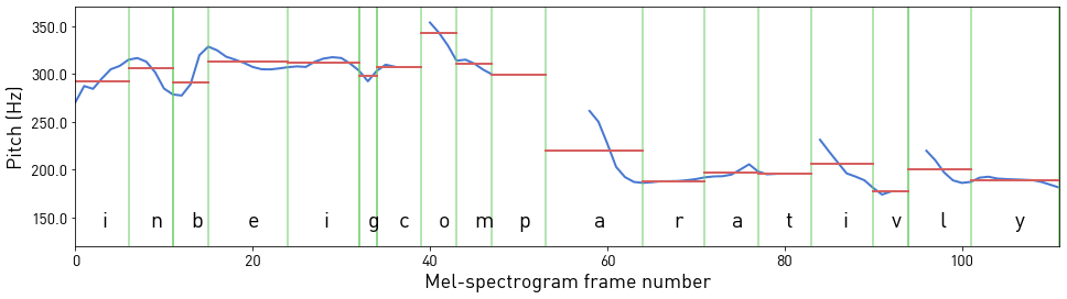
Figure 2. Pitch estimates for mel-spectrogram frames of phrase "in being comparatively" (in blue) averaged over characters (in red). Silent letters have duration 0 and are omitted.
Multi-dataset
Follow these steps to use datasets different from the default LJSpeech dataset.
-
Prepare a directory with .wav files.
./my_dataset └── wavs -
Prepare filelists with transcripts and paths to .wav files. They define training/validation split of the data (test is currently unused):
./filelists
├── my_dataset_mel_ali_pitch_text_train_filelist.txt
└── my_dataset_mel_ali_pitch_text_val_filelist.txt
Those filelists should list a single utterance per line as:
`<audio file path>|<transcript>`
The <audio file path> is the relative path to the path provided by the --dataset-path option of train.py.
- Run the pre-processing script to calculate mel-spectrograms, durations and pitch:
python extract_mels.py --cuda \
                       --dataset-path ./my_dataset \
                       --wav-text-filelist ./filelists/my_dataset_mel_ali_pitch_text_train_filelist.txt \
                       --extract-mels \
                       --extract-durations \
                       --extract-pitch-char \
                       --tacotron2-checkpoint ./pretrained_models/tacotron2/state_dict.pt"

python extract_mels.py --cuda \
                       --dataset-path ./my_dataset \
                       --wav-text-filelist ./filelists/my_dataset_mel_ali_pitch_text_val_filelist.txt \
                       --extract-mels \
                       --extract-durations \
                       --extract-pitch-char \
                       --tacotron2-checkpoint ./pretrained_models/tacotron2/state_dict.pt"
In order to use the prepared dataset, pass the following to the train.py script:
--dataset-path ./my_dataset` \
--training-files ./filelists/my_dataset_mel_ali_pitch_text_train_filelist.txt \
--validation files ./filelists/my_dataset_mel_ali_pitch_text_val_filelist.txt
Training process
FastPitch is trained to generate mel-spectrograms from raw text input. It uses short time Fourier transform (STFT) to generate target mel-spectrograms from audio waveforms to be the training targets.
The training loss is averaged over an entire training epoch, whereas the
validation loss is averaged over the validation dataset. Performance is
reported in total output mel-spectrogram frames per second and recorded as train_frames/s (after each iteration) and avg_train_frames/s (averaged over epoch) in the output log file ./output/nvlog.json.
The result is averaged over an entire training epoch and summed over all GPUs that were
included in the training.
The scripts/train.sh script is configured for 8x GPU with at least 16GB of memory:
bash --batch-size 32 --gradient-accumulation-steps 1
In a single accumulated step, there are batch_size x gradient_accumulation_steps x GPUs = 256 examples being processed in parallel. With a smaller number of GPUs, increase --gradient_accumulation_steps to keep this relation satisfied, e.g., through env variables
bash NUM_GPUS=4 GRAD_ACCUMULATION=2 bash scripts/train.sh
With automatic mixed precision (AMP), a larger batch size fits in 16GB of memory:
bash NUM_GPUS=4 GRAD_ACCUMULATION=1 BS=64 AMP=true bash scripts/train.sh
Inference process
You can run inference using the ./inference.py script. This script takes
text as input and runs FastPitch and then WaveGlow inference to produce an
audio file. It requires pre-trained checkpoints of both models
and input text as a text file, with one phrase per line.
Pre-trained FastPitch models are available for download on NGC.
Having pre-trained models in place, run the sample inference on LJSpeech-1.1 test-set with:
bash scripts/inference_example.sh
Examine the inference_example.sh script to adjust paths to pre-trained models,
and call python inference.py --help to learn all available options.
By default, synthesized audio samples are saved in ./output/audio_* folders.
FastPitch allows us to linearly adjust the pace of synthesized speech like FastSpeech.
For instance, pass --pace 0.5 for a twofold decrease in speed.
For every input character, the model predicts a pitch cue - an average pitch over a character in Hz. Pitch can be adjusted by transforming those pitch cues. A few simple examples are provided below.
| Transformation | Flag | Samples |
|---|---|---|
| - | - | link |
| Amplify pitch wrt. to the mean pitch | --pitch-transform-amplify |
link |
| Invert pitch wrt. to the mean pitch | --pitch-transform-invert |
link |
| Raise/lower pitch by | --pitch-transform-shift <hz> |
link |
| Flatten the pitch to a constant value | --pitch-transform-flatten |
link |
| Change the pace of speech (1.0 = unchanged) | --pace <value> |
link |
The flags can be combined. Modify these functions directly in the inference.py script to gain more control over the final result.
You can find all the available options by calling python inference.py --help.
More examples are presented on the website with samples.
Performance
The performance measurements in this document were conducted at the time of publication and may not reflect the performance achieved from NVIDIA’s latest software release. For the most up-to-date performance measurements, go to NVIDIA Data Center Deep Learning Product Performance.
Benchmarking
The following section shows how to run benchmarks measuring the model performance in training and inference mode.
Training performance benchmark
To benchmark the training performance on a specific batch size, run:
-
NVIDIA DGX A100 (8x A100 40GB)
AMP=true NUM_GPUS=1 BS=128 GRAD_ACCUMULATION=2 EPOCHS=10 bash scripts/train.sh AMP=true NUM_GPUS=8 BS=32 GRAD_ACCUMULATION=1 EPOCHS=10 bash scripts/train.sh NUM_GPUS=1 BS=128 GRAD_ACCUMULATION=2 EPOCHS=10 bash scripts/train.sh NUM_GPUS=8 BS=32 GRAD_ACCUMULATION=1 EPOCHS=10 bash scripts/train.sh -
NVIDIA DGX-1 (8x V100 16GB)
    AMP=true NUM_GPUS=1 BS=64 GRAD_ACCUMULATION=4 EPOCHS=10 bash scripts/train.sh
    AMP=true NUM_GPUS=8 BS=32 GRAD_ACCUMULATION=1 EPOCHS=10 bash scripts/train.sh
    NUM_GPUS=1 BS=32 GRAD_ACCUMULATION=8 EPOCHS=10 bash scripts/train.sh
    NUM_GPUS=8 BS=32 GRAD_ACCUMULATION=1 EPOCHS=10 bash scripts/train.sh
Each of these scripts runs for 10 epochs and for each epoch measures the
average number of items per second. The performance results can be read from
the nvlog.json files produced by the commands.
Inference performance benchmark
To benchmark the inference performance on a specific batch size, run:
-
For FP16
AMP=true BS_SEQUENCE=”1 4 8” REPEATS=100 bash scripts/inference_benchmark.sh -
For FP32 or TF32
BS_SEQUENCE=”1 4 8” REPEATS=100 bash scripts/inference_benchmark.sh
The output log files will contain performance numbers for the FastPitch model
(number of output mel-spectrogram frames per second, reported as generator_frames/s w )
and for WaveGlow (number of output samples per second, reported as waveglow_samples/s).
The inference.py script will run a few warm-up iterations before running the benchmark. Inference will be averaged over 100 runs, as set by the REPEATS env variable.
Results
The following sections provide details on how we achieved our performance and accuracy in training and inference.
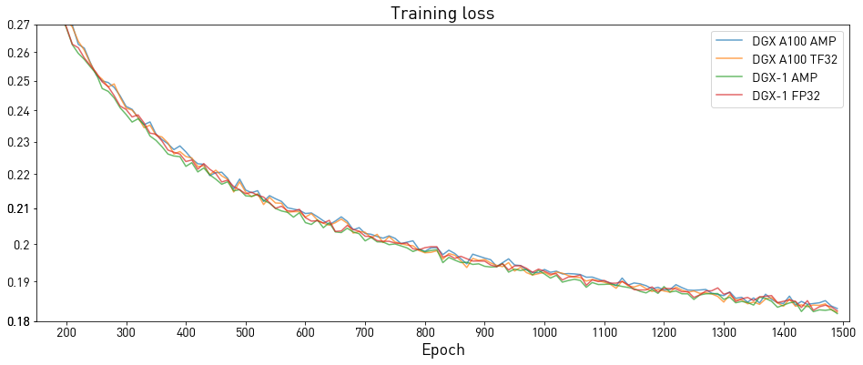
Training accuracy results
Training accuracy: NVIDIA DGX A100 (8x A100 40GB)
Our results were obtained by running the ./platform/DGXA100_FastPitch_{AMP,TF32}_8GPU.sh training script in the 20.06-py3 NGC container on NVIDIA DGX A100 (8x A100 40GB) GPUs.
| Loss (Model/Epoch) | 50 | 250 | 500 | 750 | 1000 | 1250 | 1500 |
|---|---|---|---|---|---|---|---|
| FastPitch AMP | 0.503 | 0.252 | 0.214 | 0.202 | 0.193 | 0.188 | 0.184 |
| FastPitch TF32 | 0.500 | 0.252 | 0.215 | 0.201 | 0.193 | 0.187 | 0.183 |
Training accuracy: NVIDIA DGX-1 (8x V100 16GB)
Our results were obtained by running the ./platform/DGX1_FastPitch_{AMP,FP32}_8GPU.sh training script in the PyTorch 20.06-py3 NGC container on NVIDIA DGX-1 with 8x V100 16GB GPUs.
All of the results were produced using the train.py script as described in the
Training process section of this document.
| Loss (Model/Epoch) | 50 | 250 | 500 | 750 | 1000 | 1250 | 1500 |
|---|---|---|---|---|---|---|---|
| FastPitch AMP | 0.499 | 0.250 | 0.211 | 0.198 | 0.190 | 0.184 | 0.180 |
| FastPitch FP32 | 0.503 | 0.251 | 0.214 | 0.201 | 0.192 | 0.186 | 0.182 |
Training performance results
Training performance: NVIDIA DGX A100 (8x A100 40GB)
Our results were obtained by running the ./platform/DGXA100_FastPitch_{AMP,TF32}_8GPU.sh training script in the 20.06-py3 NGC container on NVIDIA DGX A100 (8x A100 40GB) GPUs. Performance numbers, in output mel-scale spectrogram frames per second, were averaged over
an entire training epoch.
| Number of GPUs | Batch size per GPU | Frames/s with mixed precision | Frames/s with TF32 | Speed-up with mixed precision | Multi-GPU strong scaling with mixed precision | Multi-GPU strong scaling with TF32 |
|---|---|---|---|---|---|---|
| 1 | 128@AMP, 128@TF32 | 164955 | 113725 | 1.45 | 1.00 | 1.00 |
| 4 | 64@AMP, 64@TF32 | 619527 | 435951 | 1.42 | 3.76 | 3.83 |
| 8 | 32@AMP, 32@TF32 | 1040206 | 643569 | 1.62 | 6.31 | 5.66 |
Expected training time
The following table shows the expected training time for convergence for 1500 epochs:
| Number of GPUs | Batch size per GPU | Time to train with mixed precision (Hrs) | Time to train with TF32 (Hrs) | Speed-up with mixed precision |
|---|---|---|---|---|
| 1 | 128@AMP, 128@TF32 | 18.5 | 26.6 | 1.44 |
| 4 | 64@AMP, 64@TF32 | 5.5 | 7.5 | 1.36 |
| 8 | 32@AMP, 32@TF32 | 3.6 | 5.3 | 1.47 |
Training performance: NVIDIA DGX-1 (8x V100 16GB)
Our results were obtained by running the ./platform/DGX1_FastPitch_{AMP,FP32}_8GPU.sh
training script in the PyTorch 20.06-py3 NGC container on NVIDIA DGX-1 with
8x V100 16GB GPUs. Performance numbers, in output mel-scale spectrogram frames per second, were averaged over
an entire training epoch.
| Number of GPUs | Batch size per GPU | Frames/s with mixed precision | Frames/s with FP32 | Speed-up with mixed precision | Multi-GPU strong scaling with mixed precision | Multi-GPU strong scaling with FP32 |
|---|---|---|---|---|---|---|
| 1 | 64@AMP, 32@FP32 | 110370 | 41066 | 2.69 | 1.00 | 1.00 |
| 4 | 64@AMP, 32@FP32 | 402368 | 153853 | 2.62 | 3.65 | 3.75 |
| 8 | 32@AMP, 32@FP32 | 570968 | 296767 | 1.92 | 5.17 | 7.23 |
To achieve these same results, follow the steps in the Quick Start Guide.
Expected training time
The following table shows the expected training time for convergence for 1500 epochs:
| Number of GPUs | Batch size per GPU | Time to train with mixed precision (Hrs) | Time to train with FP32 (Hrs) | Speed-up with mixed precision |
|---|---|---|---|---|
| 1 | 64@AMP, 32@FP32 | 27.6 | 72.7 | 2.63 |
| 4 | 64@AMP, 32@FP32 | 8.2 | 20.3 | 2.48 |
| 8 | 32@AMP, 32@FP32 | 5.9 | 10.9 | 1.85 |
Note that most of the quality is achieved after the initial 500 epochs.
Inference performance results
The following tables show inference statistics for the FastPitch and WaveGlow text-to-speech system, gathered from 100 inference runs. Latency is measured from the start of FastPitch inference to the end of WaveGlow inference. Throughput is measured as the number of generated audio samples per second at 22KHz. RTF is the real-time factor which denotes the number of seconds of speech generated in a second of wall-clock time, per input utterance. The used WaveGlow model is a 256-channel model.
Note that performance numbers are related to the length of input. The numbers reported below were taken with a moderate length of 128 characters. Longer utterances yield higher RTF, as the generator is fully parallel.
Inference performance: NVIDIA DGX A100 (1x A100 40GB)
Our results were obtained by running the ./scripts/inference_benchmark.sh inferencing benchmarking script in the 20.06-py3 NGC container on NVIDIA DGX A100 (1x A100 40GB) GPU.
| Batch size | Precision | Avg latency (s) | Latency tolerance interval 90% (s) | Latency tolerance interval 95% (s) | Latency tolerance interval 99% (s) | Throughput (samples/sec) | Speed-up with mixed precision | Avg RTF |
|---|---|---|---|---|---|---|---|---|
| 1 | FP16 | 0.106 | 0.106 | 0.106 | 0.107 | 1,636,913 | 1.60 | 74.24 |
| 4 | FP16 | 0.390 | 0.391 | 0.391 | 0.391 | 1,780,764 | 1.55 | 20.19 |
| 8 | FP16 | 0.758 | 0.758 | 0.758 | 0.758 | 1,832,544 | 1.52 | 10.39 |
| 1 | TF32 | 0.170 | 0.170 | 0.170 | 0.170 | 1,020,894 | - | 46.30 |
| 4 | TF32 | 0.603 | 0.603 | 0.603 | 0.603 | 1,150,598 | - | 13.05 |
| 8 | TF32 | 1.153 | 1.154 | 1.154 | 1.154 | 1,202,463 | - | 6.82 |
Inference performance: NVIDIA DGX-1 (1x V100 16GB)
Our results were obtained by running the ./scripts/inference_benchmark.sh script in
the PyTorch 20.06-py3 NGC container. The input utterance has 128 characters, synthesized audio has 8.05 s.
| Batch size | Precision | Avg latency (s) | Latency tolerance interval 90% (s) | Latency tolerance interval 95% (s) | Latency tolerance interval 99% (s) | Throughput (samples/sec) | Speed-up with mixed precision | Avg RTF |
|---|---|---|---|---|---|---|---|---|
| 1 | FP16 | 0.193 | 0.194 | 0.194 | 0.194 | 902,960 | 2.35 | 40.95 |
| 4 | FP16 | 0.610 | 0.613 | 0.613 | 0.614 | 1,141,207 | 2.78 | 12.94 |
| 8 | FP16 | 1.157 | 1.161 | 1.161 | 1.162 | 1,201,684 | 2.68 | 6.81 |
| 1 | FP32 | 0.453 | 0.455 | 0.456 | 0.457 | 385,027 | - | 17.46 |
| 4 | FP32 | 1.696 | 1.703 | 1.705 | 1.707 | 411,124 | - | 4.66 |
| 8 | FP32 | 3.111 | 3.118 | 3.120 | 3.122 | 448,275 | - | 2.54 |
Inference performance: NVIDIA T4
Our results were obtained by running the ./scripts/inference_benchmark.sh script in
the PyTorch 20.06-py3 NGC container.
The input utterance has 128 characters, synthesized audio has 8.05 s.
| Batch size | Precision | Avg latency (s) | Latency tolerance interval 90% (s) | Latency tolerance interval 95% (s) | Latency tolerance interval 99% (s) | Throughput (samples/sec) | Speed-up with mixed precision | Avg RTF |
|---|---|---|---|---|---|---|---|---|
| 1 | FP16 | 0.533 | 0.540 | 0.541 | 0.543 | 326,471 | 2.56 | 14.81 |
| 4 | FP16 | 2.292 | 2.302 | 2.304 | 2.308 | 304,283 | 2.38 | 3.45 |
| 8 | FP16 | 4.564 | 4.578 | 4.580 | 4.585 | 305,568 | 1.99 | 1.73 |
| 1 | FP32 | 1.365 | 1.383 | 1.387 | 1.394 | 127,765 | - | 5.79 |
| 4 | FP32 | 5.192 | 5.214 | 5.218 | 5.226 | 134,309 | - | 1.52 |
| 8 | FP32 | 9.09 | 9.11 | 9.114 | 9.122 | 153,434 | - | 0.87 |
Release notes
We're constantly refining and improving our performance on AI and HPC workloads even on the same hardware with frequent updates to our software stack. For our latest performance data please refer to these pages for AI and HPC benchmarks.
Changelog
October 2020
- Added multispeaker capabilities
- Updated text processing module
June 2020
- Updated performance tables to include A100 results
May 2020
- Initial release
Known issues
There are no known issues with this model with this model.