33 KiB
SSD320 v1.2 For TensorFlow
This repository provides a script and recipe to train SSD320 v1.2 to achieve state of the art accuracy, and is tested and maintained by NVIDIA.
Table Of Contents
- Model overview
- Setup
- Quick Start Guide
- Advanced
- Performance
- Release notes
Model overview
The SSD320 v1.2 model is based on the SSD: Single Shot MultiBox Detector paper, which describes SSD as "a method for detecting objects in images using a single deep neural network". This model is trained with mixed precision using Tensor Cores on Volta, Turing, and the NVIDIA Ampere GPU architectures. Therefore, researchers can get results 1.5x faster than training without Tensor Cores, while experiencing the benefits of mixed precision training. This model is tested against each NGC monthly container release to ensure consistent accuracy and performance over time.
Model architecture
Our implementation is based on the existing model from the TensorFlow models repository. The network was altered in order to improve accuracy and increase throughput. Changes include:
- Replacing the VGG backbone with the more popular ResNet50.
- Adding multi-scale detection to the backbone using Feature Pyramid Networks.
- Replacing the original hard negative mining loss function with Focal Loss.
- Decreasing the input size to 320 x 320.
Default configuration
We trained the model for 12500 steps (27 epochs) with the following setup:
- SGDR with cosine decay learning rate
- Learning rate base = 0.16
- Momentum = 0.9
- Warm-up learning rate = 0.0693312
- Warm-up steps = 1000
- Batch size per GPU = 32
- Number of GPUs = 8
Feature support matrix
The following features are supported by this model:
| Feature | Transformer-XL |
|---|---|
| Automatic mixed precision (AMP) | Yes |
| Horovod Multi-GPU (NCCL) | Yes |
Features
TF-AMP - a tool that enables Tensor Core-accelerated training. Refer to the Enabling mixed precision section for more details.
Horovod - Horovod is a distributed training framework for TensorFlow, Keras, PyTorch, and MXNet. The goal of Horovod is to make distributed deep learning fast and easy to use. For more information about how to get started with Horovod, see the Horovod: Official repository.
Multi-GPU training with Horovod - our model uses Horovod to implement efficient multi-GPU training with NCCL. For details, see example sources in this repository or see the TensorFlow tutorial.
Mixed precision training
Mixed precision is the combined use of different numerical precisions in a computational method. Mixed precision training offers significant computational speedup by performing operations in half-precision format while storing minimal information in single-precision to retain as much information as possible in critical parts of the network. Since the introduction of Tensor Cores in Volta, and following with both the Turing and Ampere architectures, significant training speedups are experienced by switching to mixed precision -- up to 3x overall speedup on the most arithmetically intense model architectures. Using mixed precision training previously required two steps:
- Porting the model to use the FP16 data type where appropriate.
- Adding loss scaling to preserve small gradient values.
This can now be achieved using Automatic Mixed Precision (AMP) for TensorFlow to enablethe full mixed precision methodology in your existing TensorFlow model code. AMP enables mixed precision training on Volta and Turing GPUs automatically. The TensorFlow framework code makes all necessary model changes internally.
In TF-AMP, the computational graph is optimized to use as few casts as necessary and maximize the use of FP16, and the loss scaling is automatically applied inside of supported optimizers. AMP can be configured to work with the existing tf.contrib loss scaling manager by disabling the AMP scaling with a single environment variable to perform only the automatic mixed-precision optimization. It accomplishes this by automatically rewriting all computation graphs with the necessary operations to enable mixed precision training and automatic loss scaling.
For information about:
- How to train using mixed precision, see the Mixed Precision Training paper and Training With Mixed Precision documentation.
- Techniques used for mixed precision training, see the Mixed-Precision Training of Deep Neural Networks blog.
- How to access and enable AMP for TensorFlow, see Using TF-AMP from the TensorFlow User Guide.
Enabling mixed precision
Mixed precision is enabled in TensorFlow by using the Automatic Mixed Precision (TF-AMP) extension which casts variables to half-precision upon retrieval, while storing variables in single-precision format. Furthermore, to preserve small gradient magnitudes in backpropagation, a loss scaling step must be included when applying gradients. In TensorFlow, loss scaling can be applied statically by using simple multiplication of loss by a constant value or automatically, by TF-AMP. Automatic mixed precision makes all the adjustments internally in TensorFlow, providing two benefits over manual operations. First, programmers need not modify network model code, reducing development and maintenance effort. Second, using AMP maintains forward and backward compatibility with all the APIs for defining and running TensorFlow models.
To enable mixed precision, you can simply add the values to the environmental variables inside your training script:
-
Enable TF-AMP graph rewrite:
os.environ["TF_ENABLE_AUTO_MIXED_PRECISION_GRAPH_REWRITE"] = "1" -
Enable Automated Mixed Precision:
os.environ['TF_ENABLE_AUTO_MIXED_PRECISION'] = '1'
Enabling TF32
TensorFloat-32 (TF32) is the new math mode in NVIDIA A100 GPUs for handling the matrix math also called tensor operations. TF32 running on Tensor Cores in A100 GPUs can provide up to 10x speedups compared to single-precision floating-point math (FP32) on Volta GPUs.
TF32 Tensor Cores can speed up networks using FP32, typically with no loss of accuracy. It is more robust than FP16 for models which require high dynamic range for weights or activations.
For more information, refer to the TensorFloat-32 in the A100 GPU Accelerates AI Training, HPC up to 20x blog post.
TF32 is supported in the NVIDIA Ampere GPU architecture and is enabled by default.
Setup
The following section list the requirements in order to start training the SSD320 v1.2 model.
Requirements
This repository contains Dockerfile which extends the TensorFlow NGC container and encapsulates some dependencies. Aside from these dependencies, ensure you have the following software:
- NVIDIA Docker
- TensorFlow 20.06-py3 (or later) NGC container
- GPU-based architecture:
For more information about how to get started with NGC containers, see the following sections from the NVIDIA GPU Cloud Documentation and the Deep Learning Documentation:
- Getting Started Using NVIDIA GPU Cloud
- Accessing And Pulling From The NGC Container Registry
- Running TensorFlow
Quick Start Guide
To train your model using mixed precision or TF32 with tensor cores or using TF32, FP32, perform the following steps using the default parameters of the SSD320 v1.2 model on the COCO 2017 dataset.
1. Clone the repository.
git clone https://github.com/NVIDIA/DeepLearningExamples
cd DeepLearningExamples/TensorFlow/Detection/SSD
2. Build the SSD320 v1.2 TensorFlow NGC container.
docker build . -t nvidia_ssd
3. Download and preprocess the dataset.
Extract the COCO 2017 dataset with:
download_all.sh nvidia_ssd <data_dir_path> <checkpoint_dir_path>
Data will be downloaded, preprocessed to tfrecords format and saved in the <data_dir_path> directory (on the host).
Moreover the script will download pre-trained RN50 checkpoint in the <checkpoint_dir_path> directory
4. Launch the NGC container to run training/inference.
nvidia-docker run --rm -it --shm-size=1g --ulimit memlock=-1 --ulimit stack=67108864 -v <data_dir_path>:/data/coco2017_tfrecords -v <checkpoint_dir_path>:/checkpoints --ipc=host nvidia_ssd
5. Start training.
The ./examples directory provides several sample scripts for various GPU settings and act as wrappers around
object_detection/model_main.py script. The example scripts can be modified by arguments:
- A path to directory for checkpoints
- A path to directory for configs
- Additional arguments to
object_detection/model_main.py
If you want to run 8 GPUs, training with tensor cores acceleration and save checkpoints in /checkpoints directory, run:
bash ./examples/SSD320_FP16_8GPU.sh /checkpoints
6. Start validation/evaluation.
The model_main.py training script automatically runs validation during training.
The results from the validation are printed to stdout.
Pycocotools’ open-sourced scripts provides a consistent way to evaluate models on the COCO dataset. We are using these scripts during validation to measure models performance in AP metric. Metrics below are evaluated using pycocotools’ methodology, in the following format:during validation to measure models performance in AP metric. Metrics below are evaluated using pycocotools’ methodology, in the following format:
 Average Precision  (AP) @[ IoU=0.50:0.95 | area=   all | maxDets=100 ] = 0.273
 Average Precision  (AP) @[ IoU=0.50      | area=   all | maxDets=100 ] = 0.423
 Average Precision  (AP) @[ IoU=0.75      | area=   all | maxDets=100 ] = 0.291
 Average Precision  (AP) @[ IoU=0.50:0.95 | area= small | maxDets=100 ] = 0.024
 Average Precision  (AP) @[ IoU=0.50:0.95 | area=medium | maxDets=100 ] = 0.218
 Average Precision  (AP) @[ IoU=0.50:0.95 | area= large | maxDets=100 ] = 0.451
 Average Recall     (AR) @[ IoU=0.50:0.95 | area=   all | maxDets=  1 ] = 0.257
 Average Recall     (AR) @[ IoU=0.50:0.95 | area=   all | maxDets= 10 ] = 0.398
 Average Recall     (AR) @[ IoU=0.50:0.95 | area=   all | maxDets=100 ] = 0.427
 Average Recall     (AR) @[ IoU=0.50:0.95 | area= small | maxDets=100 ] = 0.070
 Average Recall     (AR) @[ IoU=0.50:0.95 | area=medium | maxDets=100 ] = 0.418
 Average Recall     (AR) @[ IoU=0.50:0.95 | area= large | maxDets=100 ] = 0.645
The metric reported in our results is present in the first row.
To evaluate a checkpointed model saved in the previous step, you can use script from examples directory. If you want to run inference with tensor cores acceleration, run:
bash examples/SSD320_evaluate.sh <path to checkpoint>
Advanced
The following sections provide greater details of the dataset, running training and inference, and the training results.
Scripts and sample code
Dockerfile: a container with the basic set of dependencies to run SSD
In the model/research/object_detection directory, the most important files are:
model_main.py: serves as the entry point to launch the training and inferencemodels/ssd_resnet_v1_fpn_feature_extractor.py: implementation of the modelmetrics/coco_tools.py: implementation of mAP metricutils/exp_utils.py: utility functions for running training and benchmarking
Parameters
The complete list of available parameters for the model/research/object_detection/model_main.py script contains:
./object_detection/model_main.py:
  --[no]allow_xla: Enable XLA compilation
    (default: 'false')
  --checkpoint_dir: Path to directory holding a checkpoint.  If `checkpoint_dir` is provided, this binary operates in
    eval-only mode, writing resulting metrics to `model_dir`.
  --eval_count: How many times the evaluation should be run
    (default: '1')
    (an integer)
  --[no]eval_training_data: If training data should be evaluated for this job. Note that one call only use this in eval-
    only mode, and `checkpoint_dir` must be supplied.
    (default: 'false')
  --hparams_overrides: Hyperparameter overrides, represented as a string containing comma-separated hparam_name=value
    pairs.
  --model_dir: Path to output model directory where event and checkpoint files will be written.
  --num_train_steps: Number of train steps.
    (an integer)
  --pipeline_config_path: Path to pipeline config file.
  --raport_file: Path to dlloger json
    (default: 'summary.json')
  --[no]run_once: If running in eval-only mode, whether to run just one round of eval vs running continuously (default).
    (default: 'false')
  --sample_1_of_n_eval_examples: Will sample one of every n eval input examples, where n is provided.
    (default: '1')
    (an integer)
  --sample_1_of_n_eval_on_train_examples: Will sample one of every n train input examples for evaluation, where n is
    provided. This is only used if `eval_training_data` is True.
    (default: '5')
    (an integer)
Command line options
The SSD model training is conducted by the script from the object_detection library, model_main.py.
Our experiments were done with settings described in the examples directory.
If you would like to get more details about available arguments, please run:
python object_detection/model_main.py --help
Getting the data
The SSD320 v1.2 model was trained on the COCO 2017 dataset. The val2017 validation set was used as a validation dataset.
The download_data.sh script will preprocess the data to tfrecords format.
This repository contains the download_dataset.sh script which will automatically download and preprocess the training,
validation and test datasets. By default, data will be downloaded to the /data/coco2017_tfrecords directory.
Training process
Training the SSD model is implemented in the object_detection/model_main.py script.
All training parameters are set in the config files. Because evaluation is relatively time consuming,
it does not run every epoch. By default, evaluation is executed only once at the end of the training.
The model is evaluated using pycocotools distributed with the COCO dataset.
The number of evaluations can be changed using the eval_count parameter.
To run training with tensor cores, use ./examples/SSD320_FP16_{1,4,8}GPU.sh scripts. For more details see Enabling mixed precision section below.
Data preprocessing
Before we feed data to the model, both during training and inference, we perform:
- Normalization
- Encoding bounding boxes
- Resize to 320x320
Data augmentation
During training we perform the following augmentation techniques:
- Random crop
- Random horizontal flip
- Color jitter
Enabling mixed precision
Mixed precision training offers significant computational speedup by performing operations in half-precision format, while storing minimal information in single-precision to retain as much information as possible in critical parts of the network. Since the introduction of tensor cores in the Volta and Turing architectures, significant training speedups are experienced by switching to mixed precision -- up to 3x overall speedup on the most arithmetically intense model architectures. Using mixed precision training previously required two steps:
- Porting the model to use the FP16 data type where appropriate.
- Manually adding loss scaling to preserve small gradient values.
This can now be achieved using Automatic Mixed Precision (AMP) for TensorFlow to enable the full mixed precision methodology in your existing TensorFlow model code. AMP enables mixed precision training on Volta and Turing GPUs automatically. The TensorFlow framework code makes all necessary model changes internally.
In TF-AMP, the computational graph is optimized to use as few casts as necessary and maximize the use of FP16,
and the loss scaling is automatically applied inside of supported optimizers.
AMP can be configured to work with the existing tf.contrib loss scaling manager by disabling the AMP scaling with a single environment variable to perform only the automatic mixed-precision optimization.
It accomplishes this by automatically rewriting all computation graphs with the necessary operations to enable mixed precision training and automatic loss scaling.
For information about:
- How to train using mixed precision, see the Mixed Precision Training paper and Training With Mixed Precision documentation.
- How to access and enable AMP for TensorFlow, see Using TF-AMP from the TensorFlow User Guide.
- Techniques used for mixed precision training, see the Mixed-Precision Training of Deep Neural Networks blog.
Performance
The performance measurements in this document were conducted at the time of publication and may not reflect the performance achieved from NVIDIA’s latest software release. For the most up-to-date performance measurements, go to NVIDIA Data Center Deep Learning Product Performance.
Benchmarking
The following section shows how to run benchmarks measuring the model performance in training and inference modes.
Training performance benchmark
Training benchmark was run in various scenarios on V100 16G GPU. For each scenario, batch size was set to 32.
To benchmark training, run:
bash examples/SSD320_{PREC}_{NGPU}GPU_BENCHMARK.sh
Where the {NGPU} defines number of GPUs used in benchmark, and the {PREC} defines precision.
The benchmark runs training with only 1200 steps and computes average training speed of last 300 steps.
Inference performance benchmark
Inference benchmark was run with various batch-sizes on V100 16G GPU. For inference we are using single GPU setting. Examples are taken from the validation dataset.
To benchmark inference, run:
bash examples/SSD320_FP{16,32}_inference.sh --batch_size <batch size> --checkpoint_dir <path to checkpoint>
Batch size for the inference benchmark is controlled by the --batch_size argument,
while the checkpoint is provided to the script with the --checkpoint_dir argument.
The benchmark script provides extra arguments for extra control over the experiment. We were using default values for the extra arguments during the experiments. For more details about them, please run:
bash examples/SSD320_FP16_inference.sh --help
Results
The following sections provide details on how we achieved our performance and accuracy in training and inference.
Training accuracy results
Training accuracy: NVIDIA DGX A100 (8x A100 40GB)
Our results were obtained by running the ./examples/SSD320_FP{16,32}_{1,4,8}GPU.sh script in the TensorFlow-20.06-py3 NGC container on NVIDIA DGX A100 (8x A100 40GB) GPUs.
All the results are obtained with batch size set to 32.
| Number of GPUs | Mixed precision mAP | Training time with mixed precision | TF32 mAP | Training time with TF32 |
|---|---|---|---|---|
| 1 | 0.279 | 4h 48min | 0.280 | 6h 40min |
| 4 | 0.280 | 1h 20min | 0.279 | 1h 53min |
| 8 | 0.281 | 0h 53min | 0.282 | 1h 05min |
Training accuracy: NVIDIA DGX-1 (8x V100 16GB)
Our results were obtained by running the ./examples/SSD320_FP{16,32}_{1,4,8}GPU.sh script in the TensorFlow-20.06-py3 NGC container on NVIDIA DGX-1 with 8x V100 16G GPUs.
All the results are obtained with batch size set to 32.
| Number of GPUs | Mixed precision mAP | Training time with mixed precision | FP32 mAP | Training time with FP32 |
|---|---|---|---|---|
| 1 | 0.279 | 7h 36min | 0.278 | 10h 38min |
| 4 | 0.277 | 2h 18min | 0.279 | 2h 58min |
| 8 | 0.280 | 1h 28min | 0.282 | 1h 55min |
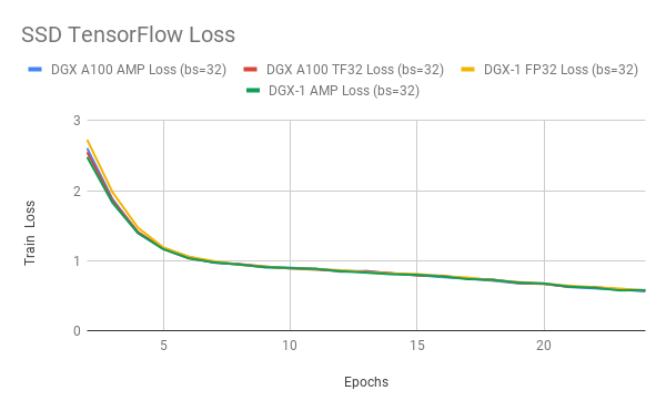
Here are example graphs of TF32, FP32 and FP16 training on 8 GPU configuration:
Training performance results
Training performance: NVIDIA DGX A100 (8x A100 40GB)
Our results were obtained by running:
python bash examples/SSD320_FP*GPU_BENCHMARK.sh
scripts in the TensorFlow-20.06-py3 NGC container on NVIDIA DGX A100 (8x A100 40GB) GPUs.
| Number of GPUs | Batch size per GPU | Mixed precision img/s | TF32 img/s | Speed-up with mixed precision | Multi-gpu weak scaling with mixed precision | Multi-gpu weak scaling with TF32 |
|---|---|---|---|---|---|---|
| 1 | 32 | 180.55 | 123.48 | 1.46 | 1.00 | 1.00 |
| 4 | 32 | 624.35 | 449.17 | 1.39 | 3.46 | 3.64 |
| 8 | 32 | 1008.46 | 779.96 | 1.29 | 5.59 | 6.32 |
To achieve same results, follow the Quick start guide outlined above.
Those results can be improved when XLA is used in conjunction with mixed precision, delivering up to 2x speedup over FP32 on a single GPU (~179 img/s). However XLA is still considered experimental.
Training performance: NVIDIA DGX-1 (8x V100 16GB)
Our results were obtained by running:
python bash examples/SSD320_FP*GPU_BENCHMARK.sh
scripts in the TensorFlow-20.06-py3 NGC container on NVIDIA DGX-1 with V100 16G GPUs.
| Number of GPUs | Batch size per GPU | Mixed precision img/s | FP32 img/s | Speed-up with mixed precision | Multi-gpu weak scaling with mixed precision | Multi-gpu weak scaling with FP32 |
|---|---|---|---|---|---|---|
| 1 | 32 | 127.96 | 84.96 | 1.51 | 1.00 | 1.00 |
| 4 | 32 | 396.38 | 283.30 | 1.40 | 3.10 | 3.33 |
| 8 | 32 | 676.83 | 501.30 | 1.35 | 5.29 | 5.90 |
To achieve same results, follow the Quick start guide outlined above.
Those results can be improved when XLA is used in conjunction with mixed precision, delivering up to 2x speedup over FP32 on a single GPU (~179 img/s). However XLA is still considered experimental.
Inference performance results
Inference performance: NVIDIA DGX A100 (1x A100 40GB)
Our results were obtained by running the examples/SSD320_FP{16,32}_inference.sh script in the TensorFlow-20.06-py3 NGC container on NVIDIA DGX A100 (1x A100 40GB) GPU.
FP16
| Batch size | Throughput Avg | Latency Avg | Latency 90% | Latency 95% | Latency 99% |
|---|---|---|---|---|---|
| 1 | 40.88 | 24.46 | 25.76 | 26.47 | 27.91 |
| 2 | 49.26 | 40.60 | 42.09 | 42.61 | 45.26 |
| 4 | 58.81 | 68.01 | 73.12 | 76.02 | 80.38 |
| 8 | 69.13 | 115.73 | 121.58 | 123.87 | 129.00 |
| 16 | 78.10 | 204.85 | 212.40 | 216.38 | 225.80 |
| 32 | 76.19 | 420.00 | 437.24 | 443.21 | 479.80 |
| 64 | 77.92 | 821.37 | 840.82 | 867.62 | 1204.64 |
TF32
| Batch size | Throughput Avg | Latency Avg | Latency 90% | Latency 95% | Latency 99% |
|---|---|---|---|---|---|
| 1 | 36.93 | 27.08 | 29.10 | 29.89 | 32.24 |
| 2 | 44.03 | 45.42 | 48.67 | 49.56 | 51.12 |
| 4 | 54.65 | 73.20 | 77.50 | 78.89 | 85.81 |
| 8 | 62.96 | 127.06 | 137.04 | 141.64 | 152.92 |
| 16 | 71.48 | 223.83 | 231.36 | 233.35 | 247.51 |
| 32 | 73.11 | 437.71 | 450.86 | 455.14 | 467.11 |
| 64 | 73.74 | 867.88 | 898.99 | 912.07 | 1077.13 |
To achieve same results, follow the Quick start guide outlined above.
Inference performance: NVIDIA DGX-1 (1x V100 16GB)
Our results were obtained by running the examples/SSD320_FP{16,32}_inference.sh script in the TensorFlow-20.06-py3 NGC container on NVIDIA DGX-1 with 1x V100 16G GPU.
FP16
| Batch size | Throughput Avg | Latency Avg | Latency 90% | Latency 95% | Latency 99% |
|---|---|---|---|---|---|
| 1 | 28.34 | 35.29 | 38.09 | 39.06 | 41.07 |
| 2 | 41.21 | 48.54 | 52.77 | 54.45 | 57.10 |
| 4 | 55.41 | 72.19 | 75.44 | 76.99 | 84.15 |
| 8 | 61.83 | 129.39 | 133.37 | 136.89 | 145.69 |
| 16 | 66.36 | 241.12 | 246.05 | 249.47 | 259.79 |
| 32 | 65.01 | 492.21 | 510.01 | 516.45 | 526.83 |
| 64 | 64.75 | 988.47 | 1012.11 | 1026.19 | 1290.54 |
FP32
| Batch size | Throughput Avg | Latency Avg | Latency 90% | Latency 95% | Latency 99% |
|---|---|---|---|---|---|
| 1 | 29.15 | 34.31 | 36.26 | 37.63 | 39.95 |
| 2 | 41.20 | 48.54 | 53.08 | 54.47 | 57.32 |
| 4 | 50.72 | 78.86 | 82.49 | 84.08 | 92.15 |
| 8 | 55.72 | 143.57 | 147.20 | 148.92 | 152.44 |
| 16 | 59.41 | 269.32 | 278.30 | 281.06 | 286.54 |
| 32 | 59.81 | 534.99 | 542.49 | 551.58 | 572.16 |
| 64 | 58.93 | 1085.96 | 1111.20 | 1118.21 | 1253.74 |
To achieve same results, follow the Quick start guide outlined above.
Inference performance: NVIDIA T4
Our results were obtained by running the examples/SSD320_FP{16,32}_inference.sh script in the TensorFlow-20.06-py3 NGC container on NVIDIA T4.
FP16
| Batch size | Throughput Avg | Latency Avg | Latency 90% | Latency 95% | Latency 99% |
|---|---|---|---|---|---|
| 1 | 19.29 | 51.90 | 53.77 | 54.95 | 59.21 |
| 2 | 30.36 | 66.04 | 70.13 | 71.49 | 73.97 |
| 4 | 37.71 | 106.21 | 111.32 | 113.04 | 118.03 |
| 8 | 40.95 | 195.49 | 201.66 | 204.00 | 210.32 |
| 16 | 41.04 | 390.05 | 399.73 | 402.88 | 410.02 |
| 32 | 40.36 | 794.48 | 815.81 | 825.39 | 841.45 |
| 64 | 40.27 | 1590.98 | 1631.00 | 1642.22 | 1838.95 |
FP32
| Batch size | Throughput Avg | Latency Avg | Latency 90% | Latency 95% | Latency 99% |
|---|---|---|---|---|---|
| 1 | 14.30 | 69.99 | 72.30 | 73.29 | 76.35 |
| 2 | 20.04 | 99.87 | 104.50 | 106.03 | 108.15 |
| 4 | 25.01 | 159.99 | 163.00 | 164.13 | 168.63 |
| 8 | 28.42 | 281.58 | 286.57 | 289.01 | 294.37 |
| 16 | 32.56 | 492.08 | 501.98 | 505.29 | 509.95 |
| 32 | 34.14 | 939.11 | 961.35 | 968.26 | 983.77 |
| 64 | 33.47 | 1915.36 | 1971.90 | 1992.24 | 2030.54 |
To achieve same results, follow the Quick start guide outlined above.
Release notes
Changelog
June 2020
- Updated performance tables to include A100 results
March 2019
- Initial release
May 2019
- Test scripts updated
Known issues
There are no known issues with this model.