42 KiB
Executable file
UNet Medical Image Segmentation for TensorFlow 2.x
This repository provides a script and recipe to train UNet Medical to achieve state of the art accuracy, and is tested and maintained by NVIDIA.
Table of Contents
- Model overview
- Setup
- Quick Start Guide
- Advanced
- Performance
- Release notes
Model overview
The UNet model is a convolutional neural network for 2D image segmentation. This repository contains a UNet implementation as described in the original paper UNet: Convolutional Networks for Biomedical Image Segmentation, without any alteration.
This model is trained with mixed precision using Tensor Cores on Volta, Turing, and the NVIDIA Ampere GPU architectures. Therefore, researchers can get results 2.2x faster than training without Tensor Cores, while experiencing the benefits of mixed precision training. This model is tested against each NGC monthly container release to ensure consistent accuracy and performance over time.
Model architecture
UNet was first introduced by Olaf Ronneberger, Philip Fischer, and Thomas Brox in the paper: UNet: Convolutional Networks for Biomedical Image Segmentation. UNet allows for seamless segmentation of 2D images, with high accuracy and performance, and can be adapted to solve many different segmentation problems.
The following figure shows the construction of the UNet model and its different components. UNet is composed of a contractive and an expanding path, that aims at building a bottleneck in its centermost part through a combination of convolution and pooling operations. After this bottleneck, the image is reconstructed through a combination of convolutions and upsampling. Skip connections are added with the goal of helping the backward flow of gradients in order to improve the training.
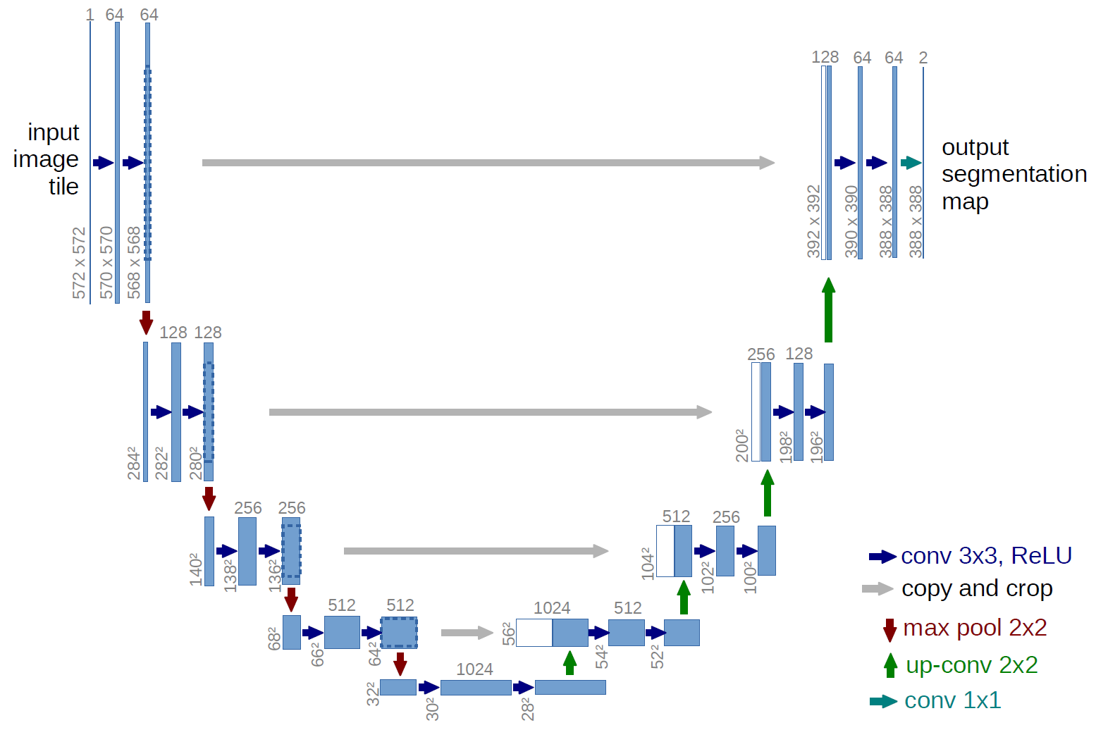 Figure 1. The architecture of a UNet model. Taken from the UNet: Convolutional Networks for Biomedical Image Segmentation paper.
Default configuration
UNet consists of a contractive (left-side) and expanding (right-side) path. It repeatedly applies unpadded convolutions followed by max pooling for downsampling. Every step in the expanding path consists of an upsampling of the feature maps and concatenation with the correspondingly cropped feature map from the contractive path.
Feature support matrix
The following features are supported by this model:
| Feature | UNet Medical |
|---|---|
| Automatic mixed precision (AMP) | Yes |
| Horovod Multi-GPU (NCCL) | Yes |
| Accelerated Linear Algebra (XLA) | Yes |
Features
Automatic Mixed Precision (AMP)
This implementation of UNet uses AMP to implement mixed precision training. It allows us to use FP16 training with FP32 master weights by modifying just a few lines of code.
Horovod
Horovod is a distributed training framework for TensorFlow, Keras, PyTorch, and MXNet. The goal of Horovod is to make distributed deep learning fast and easy to use. For more information about how to get started with Horovod, see the Horovod: Official repository.
Multi-GPU training with Horovod
Our model uses Horovod to implement efficient multi-GPU training with NCCL. For details, see example sources in this repository or see the TensorFlow tutorial.
XLA support (experimental)
XLA is a domain-specific compiler for linear algebra that can accelerate TensorFlow models with potentially no source code changes. The results are improvements in speed and memory usage: most internal benchmarks run ~1.1-1.5x faster after XLA is enabled.
Mixed precision training
Mixed precision is the combined use of different numerical precisions in a computational method. Mixed precision training offers significant computational speedup by performing operations in half-precision format while storing minimal information in single-precision to retain as much information as possible in critical parts of the network. Since the introduction of Tensor Cores in Volta, and following with both the Turing and Ampere architectures, significant training speedups are experienced by switching to mixed precision -- up to 3x overall speedup on the most arithmetically intense model architectures. Using mixed precision training previously required two steps:
- Porting the model to use the FP16 data type where appropriate.
- Adding loss scaling to preserve small gradient values.
This can now be achieved using Automatic Mixed Precision (AMP) for TensorFlow to enable the full mixed precision methodology in your existing TensorFlow model code. AMP enables mixed precision training on Volta and Turing GPUs automatically. The TensorFlow framework code makes all necessary model changes internally.
In TF-AMP, the computational graph is optimized to use as few casts as necessary and maximize the use of FP16, and the loss scaling is automatically applied inside of supported optimizers. AMP can be configured to work with the existing tf.contrib loss scaling manager by disabling the AMP scaling with a single environment variable to perform only the automatic mixed-precision optimization. It accomplishes this by automatically rewriting all computation graphs with the necessary operations to enable mixed precision training and automatic loss scaling.
For information about:
- How to train using mixed precision, see the Mixed Precision Training paper and Training With Mixed Precision documentation.
- Techniques used for mixed precision training, see the Mixed-Precision Training of Deep Neural Networks blog.
- How to access and enable AMP for TensorFlow, see Using TF-AMP from the TensorFlow User Guide.
Enabling mixed precision
This implementation exploits the TensorFlow Automatic Mixed Precision feature. To enable AMP, you simply need to supply the --amp flag to the main.py script. For reference, enabling the AMP required us to apply the following changes to the code:
-
Set Keras mixed precision policy:
if params['use_amp']: tf.keras.mixed_precision.experimental.set_policy('mixed_float16') -
Use loss scaling wrapper on the optimizer:
optimizer = tf.keras.optimizers.Adam(learning_rate=learning_rate) if using_amp: optimizer = tf.keras.mixed_precision.LossScaleOptimizer(optimizer, dynamic=True) -
Use scaled loss to calculate gradients:
scaled_loss = optimizer.get_scaled_loss(loss)
tape = hvd.DistributedGradientTape(tape)
scaled_gradients = tape.gradient(scaled_loss, model.trainable_variables)
gradients = optimizer.get_unscaled_gradients(scaled_gradients)
optimizer.apply_gradients(zip(gradients, model.trainable_variables))
Enabling TF32
TensorFloat-32 (TF32) is the new math mode in NVIDIA A100 GPUs for handling the matrix math also called tensor operations. TF32 running on Tensor Cores in A100 GPUs can provide up to 10x speedups compared to single-precision floating-point math (FP32) on Volta GPUs.
TF32 Tensor Cores can speed up networks using FP32, typically with no loss of accuracy. It is more robust than FP16 for models which require high dynamic range for weights or activations.
For more information, refer to the TensorFloat-32 in the A100 GPU Accelerates AI Training, HPC up to 20x blog post.
TF32 is supported in the NVIDIA Ampere GPU architecture and is enabled by default.
Setup
The following section lists the requirements that you need to meet in order to start training the UNet Medical model.
Requirements
This repository contains Dockerfile which extends the TensorFlow NGC container and encapsulates some dependencies. Aside from these dependencies, ensure you have the following components:
- NVIDIA Docker
- TensorFlow 21.02-tf2-py3 NGC container with Tensorflow 2.2 or later
- GPU-based architecture:
For more information about how to get started with NGC containers, see the following sections from the NVIDIA GPU Cloud Documentation and the Deep Learning Documentation:
- Getting Started Using NVIDIA GPU Cloud
- Accessing And Pulling From The NGC container registry
- Running TensorFlow
For those unable to use the TensorFlow NGC container, to set up the required environment or create your own container, see the versioned NVIDIA Container Support Matrix.
Quick Start Guide
To train your model using mixed precision with Tensor Cores or using FP32, perform the following steps using the default parameters of the UNet model on the EM segmentation challenge dataset. These steps enable you to build the UNet TensorFlow NGC container, train and evaluate your model, and generate predictions on the test data. Furthermore, you can then choose to:
- compare your evaluation accuracy with our Training accuracy results,
- compare your training performance with our Training performance benchmark,
- compare your inference performance with our Inference performance benchmark.
For the specifics concerning training and inference, see the Advanced section.
-
Clone the repository.
Executing this command will create your local repository with all the code to run UNet.
git clone https://github.com/NVIDIA/DeepLearningExamples cd DeepLearningExamples/TensorFlow2/Segmentation/UNet_Medical/ -
Build the UNet TensorFlow NGC container.
This command will use the
Dockerfileto create a Docker image namedunet_tf2, downloading all the required components automatically.docker build -t unet_tf2 .The NGC container contains all the components optimized for usage on NVIDIA hardware.
-
Start an interactive session in the NGC container to run preprocessing/training/inference.
The following command will launch the container and mount the
./datadirectory as a volume to the/datadirectory inside the container, and./resultsdirectory to the/resultsdirectory in the container.mkdir data mkdir results docker run --runtime=nvidia -it --shm-size=1g --ulimit memlock=-1 --ulimit stack=67108864 --rm --ipc=host -v ${PWD}/data:/data -v ${PWD}/results:/results unet_tf2:latest /bin/bashAny datasets and experiment results (logs, checkpoints, etc.) saved to
/dataor/resultswill be accessible in the./dataor./resultsdirectory on the host, respectively. -
Download and preprocess the data.
The UNet script
main.pyoperates on data from the ISBI Challenge, the dataset originally employed in the UNet paper. The data is available to download upon registration on the website.Training and test data are composed of 3 multi-page
TIFfiles, each containing 30 2D-images (around 30 Mb total). Once downloaded, the data can be used to run the training and benchmark scripts described below, by pointingmain.pyto its location using the--data_dirflag.Note: Masks are only provided for training data.
-
Start training.
After the Docker container is launched, the training with the default hyperparameters (for example 1/8 GPUs FP32/TF-AMP) can be started with:
bash examples/unet_TRAIN_SINGLE{_TF-AMP}.sh <number/of/gpus> <path/to/dataset> <path/to/checkpoint>For example, to run training with full precision (32-bit) on 1 GPU from the project’s folder, simply use:
bash examples/unet_TRAIN_SINGLE.sh 1 /data /results /modelThis script will launch a training on a single fold (fold 0) and store the model’s checkpoint in the <path/to/checkpoint> directory.
The script can be run directly by modifying flags if necessary, especially the number of GPUs, which is defined after the
-npflag. Since the test volume does not have labels, 20% of the training data is used for validation in 5-fold cross-validation manner. The number of fold can be changed using--foldwith an integer in range 0-4. For example, to run with 4 GPUs using fold 1 use:horovodrun -np 4 python main.py --data_dir /data --model_dir /results --batch_size 1 --exec_mode train --fold 1 --xla --ampTraining will result in a checkpoint file being written to
./resultson the host machine. -
Start validation/evaluation.
The trained model can be evaluated by passing the
--exec_mode evaluateflag. Since evaluation is carried out on a validation dataset, the--foldparameter should be filled. For example:python main.py --data_dir /data --model_dir /results --batch_size 1 --exec_mode evaluate --fold 0 --xla --ampEvaluation can also be triggered jointly after training by passing the
--exec_mode train_and_evaluateflag. -
Start inference/predictions.
The trained model can be used for inference by passing the
--exec_mode predictflag:python main.py --data_dir /data --model_dir /results --batch_size 1 --exec_mode predict --xla --ampNow that you have your model trained and evaluated, you can choose to compare your training results with our Training accuracy results. You can also choose to benchmark the performance of your training Training performance benchmark, or Inference performance benchmark. Following the steps in these sections will ensure that you achieve the same accuracy and performance results as stated in the Results section.
Advanced
The following sections provide greater details of the dataset, running training and inference, and the training results.
Scripts and sample code
In the root directory, the most important files are:
main.py: Serves as the entry point to the application.run.py: Implements the logic for training, evaluation, and inference.Dockerfile: Specifies the container with the basic set of dependencies to run UNet.requirements.txt: Set of extra requirements for running UNet.
The utils/ folder encapsulates the necessary tools to train and perform inference using UNet. Its main components are:
cmd_util.py: Implements the command-line arguments parsing.data_loader.py: Implements the data loading and augmentation.losses.py: Implements the losses used during training and evaluation.parse_results.py: Implements the intermediate results parsing.setup.py: Implements helper setup functions.
The model/ folder contains information about the building blocks of UNet and the way they are assembled. Its contents are:
layers.py: Defines the different blocks that are used to assemble UNet.unet.py: Defines the model architecture using the blocks from thelayers.pyscript.
Other folders included in the root directory are:
examples/: Provides examples for training and benchmarking UNet.images/: Contains a model diagram.
Parameters
The complete list of the available parameters for the main.py script contains:
--exec_mode: Select the execution mode to run the model (default:train). Modes available:train- trains model from scratch.evaluate- loads checkpoint (if available) and performs evaluation on validation subset (requires--foldother thanNone).train_and_evaluate- trains model from scratch and performs validation at the end (requires--foldother thanNone).predict- loads checkpoint (if available) and runs inference on the test set. Stores the results in--model_dirdirectory.train_and_predict- trains model from scratch and performs inference.
--model_dir: Set the output directory for information related to the model (default:/results).--log_dir: Set the output directory for logs (default: None).--data_dir: Set the input directory containing the dataset (default:None).--batch_size: Size of each minibatch per GPU (default:1).--fold: Selected fold for cross-validation (default:None).--max_steps: Maximum number of steps (batches) for training (default:1000).--seed: Set random seed for reproducibility (default:0).--weight_decay: Weight decay coefficient (default:0.0005).--log_every: Log performance every n steps (default:100).--learning_rate: Model’s learning rate (default:0.0001).--augment: Enable data augmentation (default:False).--benchmark: Enable performance benchmarking (default:False). If the flag is set, the script runs in a benchmark mode - each iteration is timed and the performance result (in images per second) is printed at the end. Works for bothtrainandpredictexecution modes.--warmup_steps: Used during benchmarking - the number of steps to skip (default:200). First iterations are usually much slower since the graph is being constructed. Skipping the initial iterations is required for a fair performance assessment.--xla: Enable accelerated linear algebra optimization (default:False).--amp: Enable automatic mixed precision (default:False).
Command-line options
To see the full list of available options and their descriptions, use the -h or --help command-line option, for example:
python main.py --help
The following example output is printed when running the model:
usage: main.py [-h]
              [--exec_mode {train,train_and_predict,predict,evaluate,train_and_evaluate}]
              [--model_dir MODEL_DIR] --data_dir DATA_DIR [--log_dir LOG_DIR]
              [--batch_size BATCH_SIZE] [--learning_rate LEARNING_RATE]
              [--fold FOLD]
              [--max_steps MAX_STEPS] [--weight_decay WEIGHT_DECAY]
              [--log_every LOG_EVERY] [--warmup_steps WARMUP_STEPS]
              [--seed SEED] [--augment] [--benchmark]
              [--amp] [--xla]

UNet-medical

optional arguments:
 -h, --help            show this help message and exit
 --exec_mode {train,train_and_predict,predict,evaluate,train_and_evaluate}
                       Execution mode of running the model
 --model_dir MODEL_DIR
                       Output directory for information related to the model
 --data_dir DATA_DIR   Input directory containing the dataset for training
                       the model
 --log_dir LOG_DIR     Output directory for training logs
 --batch_size BATCH_SIZE
                       Size of each minibatch per GPU
 --learning_rate LEARNING_RATE
                       Learning rate coefficient for AdamOptimizer
 --fold FOLD
                       Chosen fold for cross-validation. Use None to disable
                       cross-validation
 --max_steps MAX_STEPS
                       Maximum number of steps (batches) used for training
 --weight_decay WEIGHT_DECAY
                       Weight decay coefficient
 --log_every LOG_EVERY
                       Log performance every n steps
 --warmup_steps WARMUP_STEPS
                       Number of warmup steps
 --seed SEED           Random seed
 --augment             Perform data augmentation during training
 --benchmark           Collect performance metrics during training
 --amp                 Train using TF-AMP
 --xla                 Train using XLA
Getting the data
The UNet model uses the EM segmentation challenge dataset. Test images provided by the organization were used to produce the resulting masks for submission. The challenge's data is made available upon registration.
Training and test data are comprised of three 512x512x30 TIF volumes (test-volume.tif, train-volume.tif and train-labels.tif). Files test-volume.tif and train-volume.tif contain grayscale 2D slices to be segmented. Additionally, training masks are provided in train-labels.tif as a 512x512x30 TIF volume, where each pixel has one of two classes:
- 0 indicating the presence of cellular membrane,
- 1 corresponding to background.
The objective is to produce a set of masks that segment the data as accurately as possible. The results are expected to be submitted as a 32-bit TIF 3D image, with values between 0 (100% membrane certainty) and 1 (100% non-membrane certainty).
Dataset guidelines
The training and test datasets are given as stacks of 30 2D-images provided as a multi-page TIF that can be read using the Pillow library and NumPy (both Python packages are installed by the Dockerfile).
Initially, data is loaded from a multi-page TIF file and converted to 512x512x30 NumPy arrays with the use of Pillow. The process of loading, normalizing and augmenting the data contained in the dataset can be found in the data_loader.py script.
These NumPy arrays are fed to the model through tf.data.Dataset.from_tensor_slices(), in order to achieve high performance.
The voxel intensities then normalized to an interval [-1, 1], whereas labels are one-hot encoded for their later use in dice or pixel-wise cross-entropy loss, becoming 512x512x30x2 tensors.
If augmentation is enabled, the following set of augmentation techniques are applied:
- Random horizontal flipping
- Random vertical flipping
- Crop to a random dimension and resize to input dimension
- Random brightness shifting
In the end, images are reshaped to 388x388 and padded to 572x572 to fit the input of the network. Masks are only reshaped to 388x388 to fit the output of the network. Moreover, pixel intensities are clipped to the [-1, 1] interval.
Multi-dataset
This implementation is tuned for the EM segmentation challenge dataset. Using other datasets is possible, but might require changes to the code (data loader) and tuning some hyperparameters (e.g. learning rate, number of iterations).
In the current implementation, the data loader works with NumPy arrays by loading them at the initialization, and passing them for training in slices by tf.data.Dataset.from_tensor_slices(). If you’re able to fit your dataset into the memory, then convert the data into three NumPy arrays - training images, training labels, and testing images (optional). If your dataset is large, you will have to adapt the optimizer for the lazy-loading of data. For a walk-through, check the TensorFlow tf.data API guide
The performance of the model depends on the dataset size. Generally, the model should scale better for datasets containing more data. For a smaller dataset, you might experience lower performance.
Training process
The model trains for a total 6,400 batches (6,400 / number of GPUs), with the default UNet setup:
- Adam optimizer with learning rate of 0.0001.
This default parametrization is applied when running scripts from the ./examples directory and when running main.py without explicitly overriding these parameters. By default, the training is in full precision. To enable AMP, pass the --amp flag. AMP can be enabled for every mode of execution.
The default configuration minimizes a function L = 1 - DICE + cross entropy during training.
The training can be run directly without using the predefined scripts. The name of the training script is main.py. Because of the multi-GPU support, training should always be run with the Horovod distributed launcher like this:
horovodrun -np <number/of/gpus> python main.py --data_dir /data [other parameters]
Note: When calling the main.py script manually, data augmentation is disabled. In order to enable data augmentation, use the --augment flag in your invocation.
The main result of the training are checkpoints stored by default in ./results/ on the host machine, and in the /results in the container. This location can be controlled
by the --model_dir command-line argument, if a different location was mounted while starting the container. In the case when the training is run in train_and_predict mode, the inference will take place after the training is finished, and inference results will be stored to the /results directory.
If the --exec_mode train_and_evaluate parameter was used, and if --fold parameter is set to an integer value of {0, 1, 2, 3, 4}, the evaluation of the validation set takes place after the training is completed. The results of the evaluation will be printed to the console.
Inference process
Inference can be launched with the same script used for training by passing the --exec_mode predict flag:
python main.py --exec_mode predict --data_dir /data --model_dir <path/to/checkpoint> [other parameters]
The script will then:
- Load the checkpoint from the directory specified by the
<path/to/checkpoint>directory (/results), - Run inference on the test dataset,
- Save the resulting binary masks in a
TIFformat.
Performance
The performance measurements in this document were conducted at the time of publication and may not reflect the performance achieved from NVIDIA’s latest software release. For the most up-to-date performance measurements, go to NVIDIA Data Center Deep Learning Product Performance.
Benchmarking
The following section shows how to run benchmarks measuring the model performance in training and inference modes.
Training performance benchmark
To benchmark training, run one of the TRAIN_BENCHMARK scripts in ./examples/:
bash examples/unet_TRAIN_BENCHMARK{_TF-AMP}.sh <number/of/gpus> <path/to/dataset> <path/to/checkpoints> <batch/size>
For example, to benchmark training using mixed-precision on 8 GPUs use:
bash examples/unet_TRAIN_BENCHMARK_TF-AMP.sh 8 <path/to/dataset> <path/to/checkpoint> <batch/size>
Each of these scripts will by default run 200 warm-up iterations and benchmark the performance during training in the next 800 iterations.
To have more control, you can run the script by directly providing all relevant run parameters. For example:
horovodrun -np <num of gpus> python main.py --exec_mode train --benchmark --augment --data_dir <path/to/dataset> --model_dir <optional, path/to/checkpoint> --batch_size <batch/size> --warmup_steps <warm-up/steps> --max_steps <max/steps>
At the end of the script, a line reporting the best train throughput will be printed.
Inference performance benchmark
To benchmark inference, run one of the scripts in ./examples/:
bash examples/unet_INFER_BENCHMARK{_TF-AMP}.sh <path/to/dataset> <path/to/checkpoint> <batch/size>
For example, to benchmark inference using mixed-precision:
bash examples/unet_INFER_BENCHMARK_TF-AMP.sh <path/to/dataset> <path/to/checkpoint> <batch/size>
Each of these scripts will by default run 200 warm-up iterations and benchmark the performance during inference in the next 400 iterations.
To have more control, you can run the script by directly providing all relevant run parameters. For example:
python main.py --exec_mode predict --benchmark --data_dir <path/to/dataset> --model_dir <optional, path/to/checkpoint> --batch_size <batch/size> --warmup_steps <warm-up/steps> --max_steps <max/steps>
At the end of the script, a line reporting the best inference throughput will be printed.
Results
The following sections provide details on how we achieved our performance and accuracy in training and inference.
Training accuracy results
Training accuracy: NVIDIA DGX A100 (8x A100 80G)
The following table lists the average DICE score across 5-fold cross-validation. Our results were obtained by running the examples/unet_TRAIN_FULL{_TF-AMP}.sh training script in the tensorflow:21.02-tf2-py3 NGC container on NVIDIA DGX A100 (8x A100 80G) GPUs.
| GPUs | Batch size / GPU | DICE - TF32 | DICE - mixed precision | Time to train - TF32 | Time to train - mixed precision | Time to train speedup (TF32 to mixed precision) |
|---|---|---|---|---|---|---|
| 1 | 8 | 0.8900 | 0.8902 | 21.3 | 8.6 | 2.48 |
| 8 | 8 | 0.8855 | 0.8858 | 2.5 | 2.5 | 1.00 |
Training accuracy: NVIDIA DGX-1 (8x V100 16G)
The following table lists the average DICE score across 5-fold cross-validation. Our results were obtained by running the examples/unet_TRAIN_FULL{_TF-AMP}.sh training script in the tensorflow:21.02-tf2-py3 NGC container on NVIDIA DGX-1 with (8x V100 16G) GPUs.
| GPUs | Batch size / GPU | DICE - FP32 | DICE - mixed precision | Time to train - FP32 [min] | Time to train - mixed precision [min] | Time to train speedup (FP32 to mixed precision) |
|---|---|---|---|---|---|---|
| 1 | 8 | 0.8901 | 0.8898 | 47 | 16 | 2.94 |
| 8 | 8 | 0.8848 | 0.8857 | 7 | 4.5 | 1.56 |
To reproduce this result, start the Docker container interactively and run one of the TRAIN scripts:
bash examples/unet_TRAIN_FULL{_TF-AMP}.sh <number/of/gpus> <path/to/dataset> <path/to/checkpoint> <batch/size>
for example
bash examples/unet_TRAIN_FULL_TF-AMP.sh 8 /data /results 8
This command will launch a script which will run training on 8 GPUs for 6400 iterations five times for 5-fold cross-validation.
At the end, it will collect the scores and print the average validation DICE score and cross-entropy loss.
The time reported is for one fold, which means that the training for 5 folds will take 5 times longer.
The default batch size is 8, however if you have less than 16 Gb memory card and you encounter GPU memory issue you should decrease the batch size.
The logs of the runs can be found in /results directory once the script is finished.
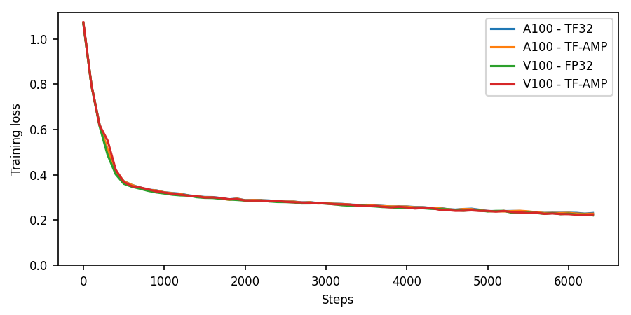
Learning curves
The following image show the training loss as a function of iteration for training using DGX A100 (TF32 and TF-AMP) and DGX-1 V100 (FP32 and TF-AMP).
Training performance results
Training performance: NVIDIA DGX A100 (8x A100 80G)
Our results were obtained by running the examples/unet_TRAIN_BENCHMARK{_TF-AMP}.sh training script in the NGC container on NVIDIA DGX A100 (8x A100 80G) GPUs. Performance numbers (in images per second) were averaged over 1000 iterations, excluding the first 200 warm-up steps.
| GPUs | Batch size / GPU | Throughput - TF32 [img/s] | Throughput - mixed precision [img/s] | Throughput speedup (TF32 - mixed precision) | Weak scaling - TF32 | Weak scaling - mixed precision |
|---|---|---|---|---|---|---|
| 1 | 1 | 46.88 | 75.04 | 1.60 | - | - |
| 1 | 8 | 63.33 | 141.03 | 2.23 | - | - |
| 8 | 1 | 298.91 | 384.27 | 1.29 | 6.37 | 5.12 |
| 8 | 8 | 470.50 | 1000.89 | 2.13 | 7.43 | 7.10 |
Training performance: NVIDIA DGX-1 (8x V100 16G)
Our results were obtained by running the examples/unet_TRAIN_BENCHMARK{_TF-AMP}.sh training script in the tensorflow:21.02-tf2-py3 NGC container on NVIDIA DGX-1 with (8x V100 16G) GPUs. Performance numbers (in images per second) were averaged over 1000 iterations, excluding the first 200 warm-up steps.
| GPUs | Batch size / GPU | Throughput - FP32 [img/s] | Throughput - mixed precision [img/s] | Throughput speedup (FP32 - mixed precision) | Weak scaling - FP32 | Weak scaling - mixed precision |
|---|---|---|---|---|---|---|
| 1 | 1 | 16.92 | 39.63 | 2.34 | - | - |
| 1 | 8 | 19.40 | 60.65 | 3.12 | - | - |
| 8 | 1 | 120.90 | 225.27 | 1.86 | 7.14 | 5.68 |
| 8 | 8 | 137.11 | 419.99 | 3.06 | 7.07 | 6.92 |
To achieve these same results, follow the steps in the Training performance benchmark section.
Throughput is reported in images per second. Latency is reported in milliseconds per image.
TensorFlow 2 runs by default using the eager mode, which makes tensor evaluation trivial at the cost of lower performance. To mitigate this issue multiple layers of performance optimization were implemented. Two of them, AMP and XLA, were already described. There is an additional one called Autograph, which allows to construct a graph from a subset of Python syntax improving the performance simply by adding a @tf.function decorator to the train function. To read more about Autograph see Better performance with tf.function and AutoGraph.
Inference performance results
Inference performance: NVIDIA DGX A100 (1x A100 80G)
Our results were obtained by running the examples/unet_INFER_BENCHMARK{_TF-AMP}.sh inference benchmarking script in the tensorflow:21.02-tf2-py3 NGC container on NVIDIA DGX A100 (1x A100 80G) GPU.
FP16
| Batch size | Resolution | Throughput Avg [img/s] | Latency Avg [ms] | Latency 90% [ms] | Latency 95% [ms] | Latency 99% [ms] |
|---|---|---|---|---|---|---|
| 1 | 572x572x1 | 275.98 | 3.534 | 3.543 | 3.544 | 3.547 |
| 2 | 572x572x1 | 376.68 | 10.603 | 10.619 | 10.623 | 10.629 |
| 4 | 572x572x1 | 443.05 | 19.572 | 19.610 | 19.618 | 19.632 |
| 8 | 572x572x1 | 440.71 | 19.386 | 19.399 | 19.401 | 19.406 |
| 16 | 572x572x1 | 462.79 | 37.760 | 37.783 | 37.788 | 37.797 |
TF32
| Batch size | Resolution | Throughput Avg [img/s] | Latency Avg [ms] | Latency 90% [ms] | Latency 95% [ms] | Latency 99% [ms] |
|---|---|---|---|---|---|---|
| 1 | 572x572x1 | 152.27 | 9.317 | 9.341 | 9.346 | 9.355 |
| 2 | 572x572x1 | 180.84 | 17.294 | 17.309 | 17.312 | 17.318 |
| 4 | 572x572x1 | 203.60 | 31.676 | 31.698 | 31.702 | 31.710 |
| 8 | 572x572x1 | 208.70 | 57.742 | 57.755 | 57.757 | 57.762 |
| 16 | 572x572x1 | 213.15 | 112.545 | 112.562 | 112.565 | 112.572 |
To achieve these same results, follow the steps in the Quick Start Guide.
Inference performance: NVIDIA DGX-1 (1x V100 16G)
Our results were obtained by running the examples/unet_INFER_BENCHMARK{_TF-AMP}.sh inference benchmarking script in the tensorflow:21.02-tf2-py3 NGC container on NVIDIA DGX-1 with (1x V100 16G) GPU.
FP16
| Batch size | Resolution | Throughput Avg [img/s] | Latency Avg [ms] | Latency 90% [ms] | Latency 95% [ms] | Latency 99% [ms] |
|---|---|---|---|---|---|---|
| 1 | 572x572x1 | 142.15 | 10.537 | 6.851 | 6.853 | 6.856 |
| 2 | 572x572x1 | 159.25 | 13.230 | 13.242 | 13.244 | 13.248 |
| 4 | 572x572x1 | 178.19 | 26.035 | 26.049 | 26.051 | 26.057 |
| 8 | 572x572x1 | 188.54 | 43.602 | 43.627 | 43.631 | 43.640 |
| 16 | 572x572x1 | 195.27 | 85.743 | 85.807 | 85.819 | 85.843 |
FP32
| Batch size | Resolution | Throughput Avg [img/s] | Latency Avg [ms] | Latency 90% [ms] | Latency 95% [ms] | Latency 99% [ms] |
|---|---|---|---|---|---|---|
| 1 | 572x572x1 | 51.71 | 20.065 | 20.544 | 20.955 | 21.913 |
| 2 | 572x572x1 | 55.87 | 37.112 | 37.127 | 37.130 | 37.136 |
| 4 | 572x572x1 | 58.15 | 73.033 | 73.068 | 73.074 | 73.087 |
| 8 | 572x572x1 | 59.28 | 144.829 | 144.924 | 144.943 | 144.979 |
| 16 | 572x572x1 | 73.01 | 234.995 | 235.098 | 235.118 | 235.157 |
To achieve these same results, follow the steps in the Inference performance benchmark section.
Throughput is reported in images per second. Latency is reported in milliseconds per batch.
Release notes
Changelog
February 2021
- Updated training and inference performance with V100 and A100 results
- Refactored the example scripts
June 2020
- Updated training and inference accuracy with A100 results
- Updated training and inference performance with A100 results
February 2020
- Initial release
Known issues
- Training on 8 GPUs with FP32 and XLA using batch size 8 may sometimes cause out-of-memory errors.
- For TensorFlow 2.0 the training performance using AMP and XLA is around 30% lower than reported here. The issue was solved in TensorFlow 2.1.